On this page
Most students first meet compound interest as a formula to memorise: A = P(1 + r/100)ⁿ. Yet memorising this equation without understanding where it comes from turns financial mathematics into arbitrary symbols. In reality, the formula is nothing more than repeated simple interest where the interest earned at the end of each period is rolled into the principal for the next. By following this process year by year, you can see how the exponent n appears naturally as a repeated multiplier rather than an abstract rule.
How do you derive the compound interest formula year by year?
To derive the formula from first principles, imagine depositing a principal sum P at an annual interest rate of r% per annum compounded annually. The derivation, detailed in the NCERT Class 8 Mathematics curriculum under Comparing Quantities, treats each single year as a standard simple interest calculation. If you need a refresher on the base components, see our guide on how to find principal, rate, or time in simple interest.
For the first year:
The initial principal is P₁ = P.
The simple interest earned in Year 1 is SI₁ = (P × r × 1) / 100 = Pr / 100.
The total amount at the end of Year 1 is A₁ = P + SI₁ = P + (Pr / 100) = P(1 + r/100).
For the second year, the key transition occurs: the accumulated amount A₁ becomes the new starting principal P₂.
The new principal is P₂ = A₁ = P(1 + r/100).
The interest earned in Year 2 is SI₂ = (P₂ × r × 1) / 100 = P(1 + r/100) × (r / 100).
The amount at the end of Year 2 is A₂ = P₂ + SI₂ = P(1 + r/100) + [P(1 + r/100) × (r / 100)].
Now factor out the common term P(1 + r/100): A₂ = P(1 + r/100) × [1 + r/100] = P(1 + r/100)².
For the third year, the pattern repeats directly. The starting principal P₃ is A₂ = P(1 + r/100)². Adding the interest earned in Year 3 and factoring out P(1 + r/100)² produces: A₃ = P(1 + r/100)³.
Observing this progression reveals that at the end of year n, the accumulated amount A is: A = P(1 + r/100)ⁿ.
Because the amount represents principal plus accumulated interest, the net compound interest (CI) is found by subtracting the starting principal: CI = A − P = P[(1 + r/100)ⁿ − 1].
When working through multi-stage arithmetic or algebraic proofs, the Fermi Problem Library provides worked problems with a step-by-step solver that explains the reasoning rather than printing an answer.
How does the year-by-year calculation work with real numbers?
To verify that the algebraic formula matches real-world arithmetic, consider a concrete numerical example. Suppose you deposit P = ₹10,000 at an interest rate of r = 10% per annum for n = 3 years, as framed in standard classroom exercises in the NCERT Class 8 Mathematics curriculum.
Walking through the yearly arithmetic shows the step-by-step accumulation:
Year 1: Starting principal is ₹10,000. Interest earned is (10,000 × 10 × 1) / 100 = ₹1,000. The ending amount A₁ is ₹10,000 + ₹1,000 = ₹11,000.
Year 2: Starting principal becomes ₹11,000. Interest earned is (11,000 × 10 × 1) / 100 = ₹1,100. The ending amount A₂ is ₹11,000 + ₹1,100 = ₹12,100.
Year 3: Starting principal becomes ₹12,100. Interest earned is (12,100 × 10 × 1) / 100 = ₹1,210. The ending amount A₃ is ₹12,100 + ₹1,210 = ₹13,310.
Total compound interest earned over the 3-year term is ₹13,310 − ₹10,000 = ₹3,310.
Now evaluate the closed-form formula for the same parameters: A = 10,000 × (1 + 10/100)³ = 10,000 × (1.10)³ = 10,000 × 1.331 = ₹13,310.
Both approaches yield the exact same total of ₹13,310. The closed-form formula condenses three separate calculations into one algebraic step, making it indispensable when time spans extend to 10 or 20 years.
How does compound interest differ from simple interest over time?
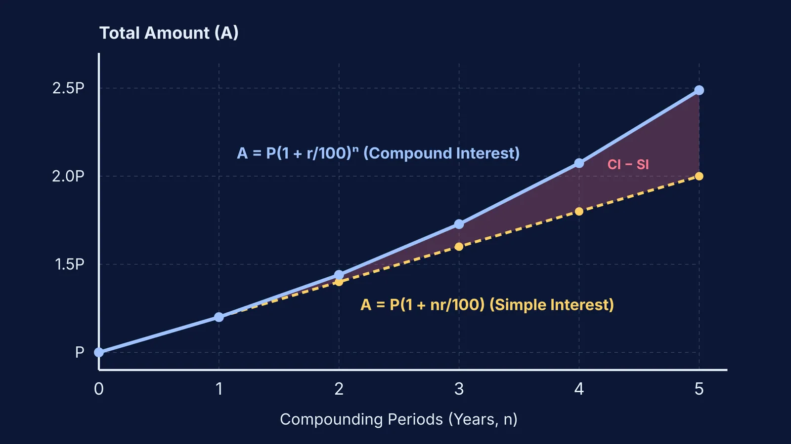
The defining characteristic of compound interest is that interest earns interest. Under simple interest, the annual interest is calculated solely on the original principal P, meaning the payout remains flat every single year. According to financial definitions documented on Wikipedia, simple interest grows linearly while compound interest grows exponentially.
Comparing the same deposit of ₹10,000 at 10% per annum over 3 years clarifies the divergence:
Simple interest total: SI = (10,000 × 10 × 3) / 100 = ₹3,000. The total simple amount is ₹10,000 + ₹3,000 = ₹13,000.
Compound interest total: As calculated above, the compound amount is ₹13,310, yielding a net interest of ₹3,310.
Net difference: CI − SI = ₹13,310 − ₹13,000 = ₹310.
Where does this extra ₹310 come from? It represents interest earned on previously accumulated interest:
In Year 2: The extra ₹1,000 earned in Year 1 generates 10% interest, contributing ₹100.
In Year 3: The initial ₹1,000 from Year 1 generates another ₹100, while the ₹1,100 from Year 2 generates ₹110 (comprising ₹100 on the base plus ₹10 on Year 2's extra interest).
Summing these extra gains gives ₹100 + ₹100 + ₹110 = ₹310.
In the first year, simple interest and compound interest are identical because no previous interest exists to compound. By year two and three, the gap opens up. For a closer look at the algebraic shortcut for this gap, read our analysis of the difference between compound and simple interest for two years.
What happens when interest compounds half-yearly or quarterly?
The year-by-year derivation easily adapts when compounding occurs more frequently than once a year. When a financial institution compounds interest half-yearly, there are two compounding conversion periods each year. Following standard conventions in the NCERT Class 8 Mathematics syllabus, the annual interest rate r is halved to r/2, and the number of periods is doubled to 2n.
The generalized compounding formula, as formalized in college texts such as OpenStax College Algebra, becomes: A = P[1 + r / (100 × m)]^(m × n)
where m represents the number of compounding cycles per year:
Compounded annually: m = 1
Compounded half-yearly: m = 2, so A = P(1 + r/200)^(2n)
Compounded quarterly: m = 4, so A = P(1 + r/400)^(4n)
This same multiplicative structure extends well beyond banking. It governs biological population growth and asset depreciation, as discussed in our guide to population growth and depreciation formulas. For students moving from school algebra to competitive entrance mathematics, the Fermi Concept Library covers every concept in physics, chemistry, biology, mathematics and computing, each with its own lesson and its place in the map.