On this page
When comparing two distributions, looking only at the standard deviation can be misleading. If two series have very different means, a direct comparison of their absolute spreads will often lead you to the wrong conclusion.
To answer the question of which series is more variable, you need a relative measure.
Why is standard deviation not always enough?
Before jumping to the coefficient of variation, it helps to understand why the standard deviation alone falls short. Standard deviation measures the absolute distance that data points fall from the mean. It is measured in the exact same units as the original data—runs, kilograms, or metres.
If you are comparing two factories that produce steel rods of the same average length, the standard deviation is a perfect tool. The factory with the lower standard deviation is more consistent. But when the two groups you are comparing have drastically different averages, the absolute spread becomes misleading. A variation of one kilogram is insignificant if you are weighing an elephant, but it is a massive error if you are weighing a mouse.
This is exactly why statisticians use a relative measure. By dividing the absolute spread by the mean, you cancel out the units and the scale. This leaves a pure percentage that can be compared fairly across any two distributions.
What is the coefficient of variation?
The coefficient of variation (CV) is a statistical measure of relative dispersion. It is calculated by dividing the standard deviation (σ) by the mean (x̄), and it is often multiplied by 100 to be expressed as a percentage.
Because it is a ratio of two quantities with the same units, the CV is a dimensionless number 1. This scale invariance allows you to compare the relative volatility of datasets that have widely different means or even entirely different units 1.
Which series is more variable?
The rule of thumb in statistics is simple: the series having a greater coefficient of variation is said to be more variable 1. Conversely, the series with the lower CV is considered more consistent.
Imagine you are a cricket selector comparing the scores of two batsmen over five innings:
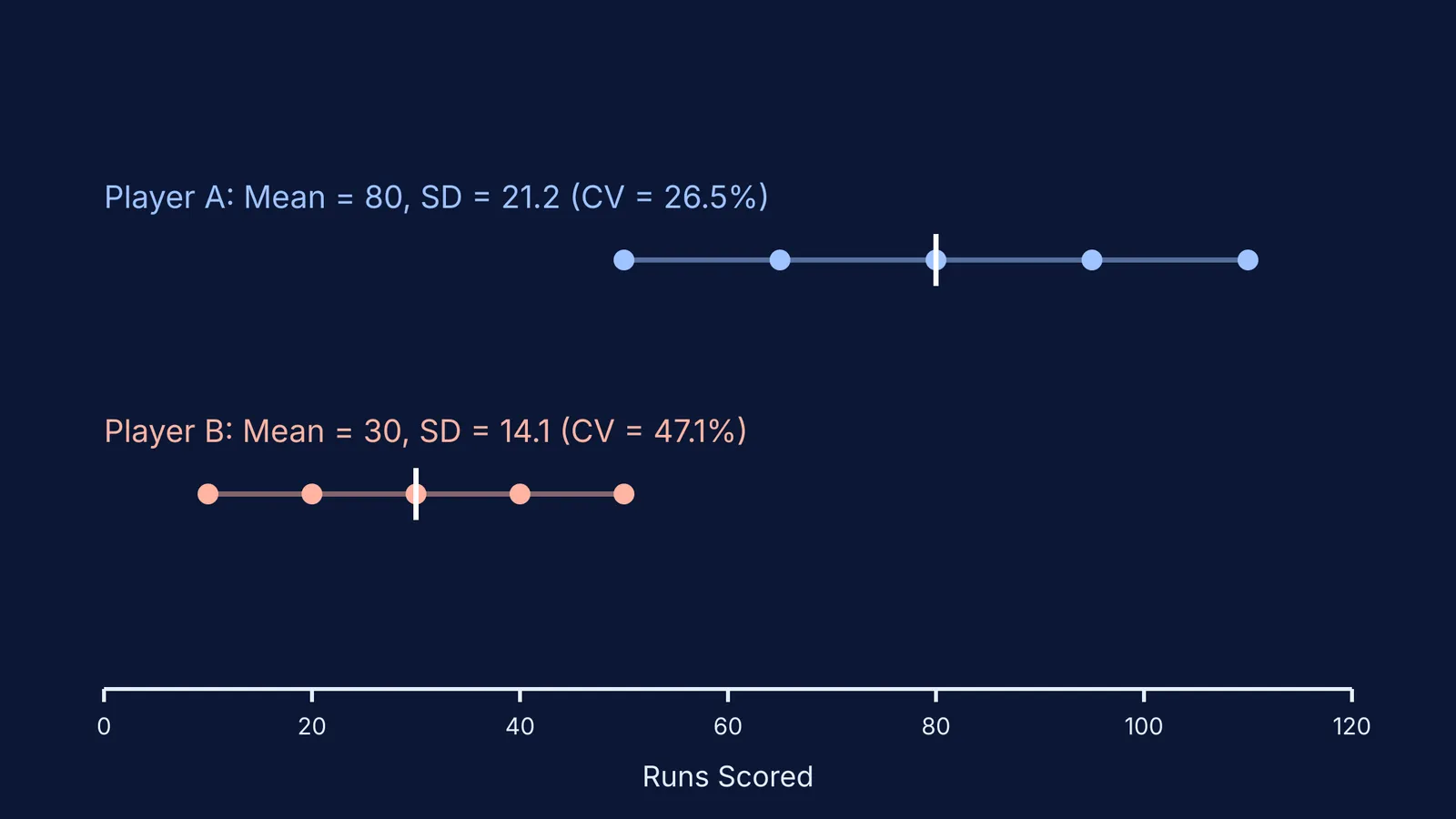
Player A (The Anchor): Scores of 50, 65, 80, 95, and 110 runs.
Player B (The Tail-ender): Scores of 10, 20, 30, 40, and 50 runs.
First, we find the mean (x̄) for both players. Player A has scored 400 runs across 5 innings, giving a mean of 80. Player B has scored 150 runs across 5 innings, giving a mean of 30.
Next, we calculate the standard deviation (σ). Player A's scores deviate from their mean by 30, 15, 0, 15, and 30 runs. Squaring these differences gives 900, 225, 0, 225, and 900. The average of these squares (the variance) is 450. The square root of 450 gives Player A a standard deviation of 21.2 runs.
Following the same process for Player B, the deviations from their mean of 30 are 20, 10, 0, 10, and 20. Squaring these gives 400, 100, 0, 100, and 400. The variance is 200, and the square root of 200 gives a standard deviation of 14.1 runs.
If you only look at the absolute standard deviation, Player B (14.1 runs) appears more consistent than Player A (21.2 runs). A 14-run swing is massive for a player who only averages 30 runs—it represents almost half their typical score. Meanwhile, a 21-run swing is relatively small for a player who averages a massive 80 runs.
To find out exactly which series is more variable, we calculate the coefficient of variation for each.
For Player A: CV = (21.2 / 80) × 100 = 26.5% 1
For Player B: CV = (14.1 / 30) × 100 = 47.1% 1
Player B has the higher CV, which means Player B's scores are more variable relative to their average. Player A is therefore the more consistent batsman, despite having a larger absolute standard deviation.
How do you calculate the coefficient of variation?
If you are solving Class 11 statistics problems by hand, a methodical approach prevents arithmetic errors from ruining your final comparison.
Calculate the mean (x̄): Add all the values together and divide by the number of observations. For grouped data, use the sum of products of frequencies and class marks.
Calculate the deviations: Subtract the mean from each individual value to find the deviation.
Square the deviations: Square each result to eliminate negative signs.
Find the variance: Calculate the average of these squared deviations.
Find the standard deviation (σ): Take the square root of the variance.
Calculate the CV: Divide the standard deviation by the mean and multiply by 100.
The final step is to compare the two percentages. The series with the greater percentage is more variable.
How to use AI to check variability?
When revising for exams, checking long statistical calculations by hand can be frustrating. A single misplaced decimal point in the variance calculation will break the final CV ratio.
This is where the Fermi Problem Library comes in. Rather than printing an answer, it has worked problems with a step-by-step solver that explains the reasoning. You can bring a problem set featuring two distributions, and the AI tutor will explain how the standard deviation is derived before using it to compare them. If you get stuck on an earlier step, such as finding the missing observation from a mean, the tutor will break it down further.
For more foundational tools used in data handling, you can also explore the rules for choosing a bar graph vs histogram and review the basic statistics every student science project needs.