

On this page
It is a classic mistake in statistics exams: drawing separate bars when the data demands a continuous block, or using raw counts as heights when the bin widths change. Though they look similar at first glance, bar graphs and histograms follow completely different mathematical rules and serve entirely different purposes.
Here is exactly how to tell them apart, when to use each, and how to successfully navigate the trap of unequal class widths.
What is the difference between a bar graph and a histogram?
The central distinction between the two charts comes down to the fundamental type of data you are attempting to plot.
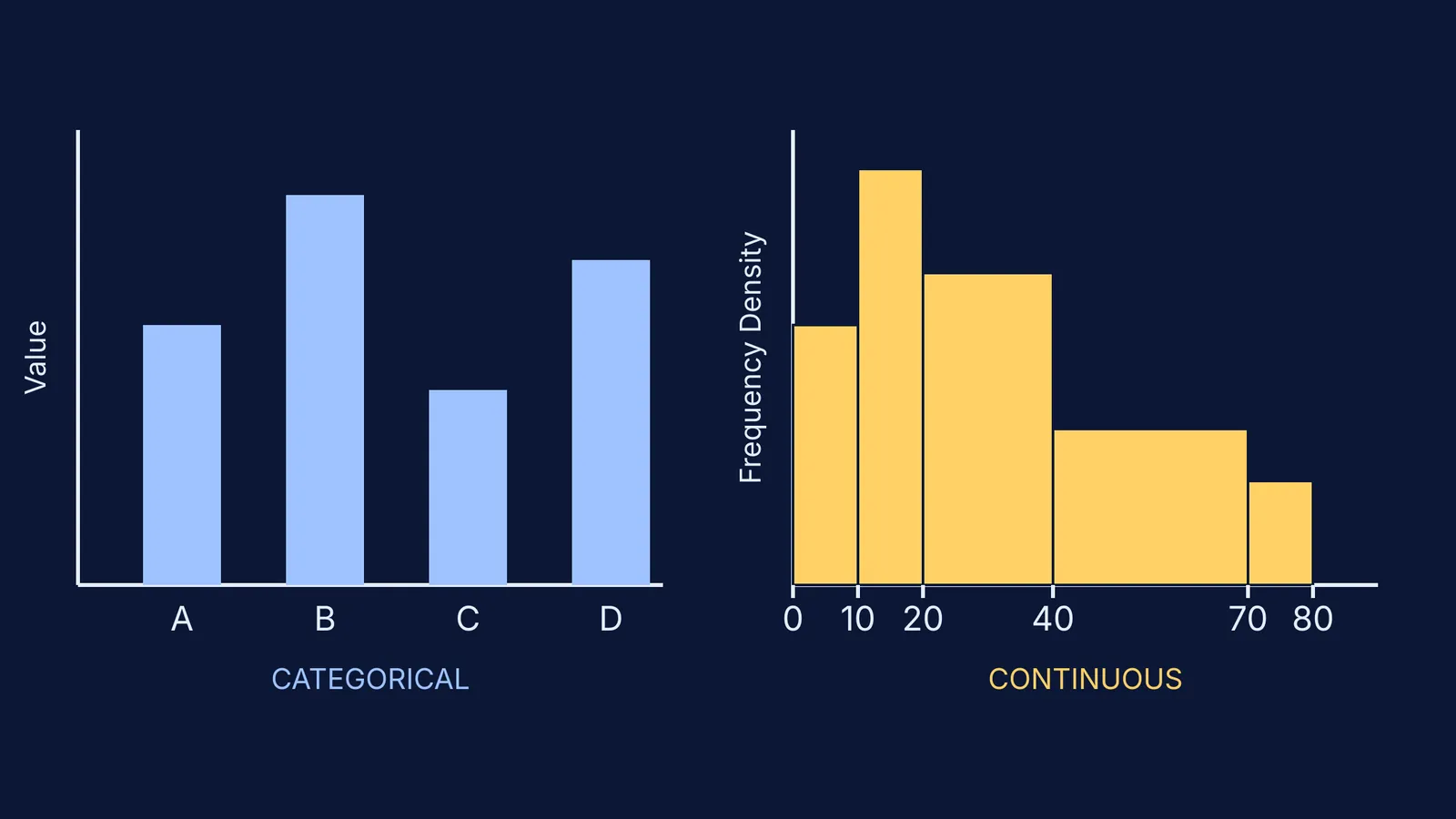
A bar graph (or bar chart) represents categorical or discrete data. If you are plotting the number of students who prefer apples, mangoes, or grapes, each fruit represents a category that is entirely separate from the others. The Scottish engineer William Playfair published the first known bar chart in 1786 to show imports and exports (Wikipedia). In a standard bar graph, the order of the bars does not mathematically matter—you could alphabetise them or sort them by size without changing the meaning of the chart. Most importantly, the height of the bar is directly proportional to the value or frequency it represents.
A histogram, on the other hand, represents continuous numerical data that has been grouped into specific intervals (sometimes called bins). If you are plotting the heights of students in a class (for example, 140–150 cm, and 150–160 cm), the data flows continuously from one interval to the next. The English mathematician Karl Pearson introduced the term "histogram" in 1892 to describe this specific form of graphical representation (Wikipedia).
You can explore more statistics fundamentals in the Fermi Concept Library, which maps out every concept in mathematics.
Why do histograms have no gaps?
Because a bar graph deals with discrete, independent categories, you must draw equal gaps between consecutive bars. These physical gaps on the paper signal to the reader that the categories do not bleed into one another.
Because a histogram deals with a continuous number line along the x-axis, there are no gaps between the bars. The upper limit of one class interval is exactly the lower limit of the next interval. The bars must touch to demonstrate that every possible value in the continuous range is accounted for, leaving no numbers out.
If you are stuck on whether your data is continuous or categorical, Fermi's AI tutor can work out what you already know and build a plan for the session, teaching you the difference through interactive examples.
How do you adjust heights for unequal class widths?
This is the most common place students lose marks in examinations. In a bar graph, all bars typically have the same width, and that width means absolutely nothing mathematically. But in a histogram, the width of the bar represents the size of the class interval.
In a mathematically correct histogram, the area of each rectangle—not merely its height—must be proportional to the frequency of the interval (Wikipedia).
If all your class intervals are perfectly equal (such as 0–10, 10–20, and 20–30), you can simply plot the raw frequency as the height. However, if the examiner gives you unequal class widths (such as 0–10, 10–20, and 20–40), plotting raw frequency as height creates a visually distorted graph where wide bars look artificially massive and exaggerate the data.
To fix this visual distortion, you must calculate and plot the frequency density on the y-axis:
Frequency Density = Frequency ÷ Class Width
A worked example of unequal class widths
Imagine you are given this data for test scores across a class:
0 to 10: The frequency is 5. The class width is 10.
Frequency Density = 5 ÷ 10 = 0.5
10 to 20: The frequency is 8. The class width is 10.
Frequency Density = 8 ÷ 10 = 0.8
20 to 40: The frequency is 12. The class width is 20.
Frequency Density = 12 ÷ 20 = 0.6
40 to 70: The frequency is 9. The class width is 30.
Frequency Density = 9 ÷ 30 = 0.3
Notice that while the 20–40 interval has the highest total frequency of students (12), the 10–20 interval actually has the highest frequency density (0.8). When you draw the final histogram, the 10–20 bar will be the tallest, accurately showing where the test scores are most densely packed.
If you need to practice problems exactly like this one, the Fermi Problem Library has worked problems with a step-by-step solver that explains the reasoning rather than printing an answer.
By double-checking for continuity and always watching out for unequal widths, you ensure your statistical graphs tell the true and accurate story of the data.
Read more:


