

On this page
When preparing an investigatory science project or school survey, the easiest mistake is reporting only an average. Testing a fertilizer on three seedlings or surveying ten classmates about study hours gives a mean, but an average without spread hides whether results were steady or erratic. If three seedlings grow 12 cm, 2 cm, and 7 cm, their mean is 7 cm. If three others all grow 7 cm, their mean is also 7 cm. The averages match, yet the first reflects wide variation while the second shows consistent growth. In our guide on turning a curious question into a fair experiment, controlled variables only matter if measurements prove the result was not an accident.
Why is a single average not enough for a project?
To describe data honestly, every project must report spread alongside the mean. The standard deviation measures how far individual observations sit from the average. In our primer on mean, variance and standard deviation, squared deviations show whether readings cluster tightly or scatter widely. Pairing the mean with the standard deviation proves that you measured variability rather than cherry-picking one favourable trial.
What is the difference between standard deviation and standard error?
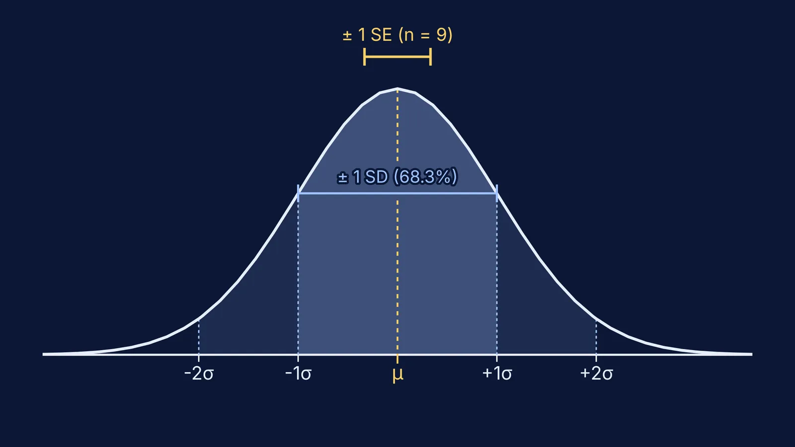
Students and researchers frequently confuse standard deviation (SD) with standard error of the mean (SE). In a 2007 paper in *The Journal of Cell Biology*, Geoff Cumming, Fiona Fidler, and David L. Vaux (doi:10.1083/jcb.200611141) showed that standard deviation is descriptive: it reflects natural spread among individual observations and does not shrink when you collect more data. In contrast, standard error is inferential: it estimates how closely your sample average reflects the true population mean, calculated as SE = SD / √n, where n is sample size.
As Martin Krzywinski and Naomi Altman explained in *Nature Methods* (doi:10.1038/nmeth.2659), standard error shrinks as sample size grows because larger samples yield a more stable mean. A common misconception is that standard error bars must merely not overlap to establish significance at p < 0.05. In fact, if two standard error bars just touch, p is roughly 0.17; for independent groups of ten or more observations, the bars must be separated by a gap of about one standard error arm to indicate p < 0.05. Cumming and his co-authors emphasized that figures must explicitly state what error bars represent and report sample size n.
For step-by-step guidance on calculating variance, standard deviation, and pooled datasets, the Fermi Problem Library explains the underlying reasoning rather than just printing an answer.
How many samples or repeated trials do you need?
For school physics and chemistry experiments, recording three to five repeated trials per condition guards against accidental measurement slips. For biological specimens or surveys where variability is high, three trials rarely support firm conclusions. In *Nature Methods* (doi:10.1038/nmeth.2738), Martin Krzywinski and Naomi Altman showed that underpowered studies with small sample sizes frequently miss real effects or exaggerate findings. As shown in our review of Ronald Fisher's principles of experimental design, replication and randomisation turn a demonstration into valid science.
The American Statistical Association's GAISE II framework (doi:10.5951/mtlt.2020.0343) urges students to move past rigid rules like "n must equal 30" and assess the source of variation. Polling 15 classmates at lunch is a convenience sample loaded with bias; 40 to 60 students sampled across different classes provides a much fairer survey picture.
If you want to see how sample size alters distributions and shrinks sampling uncertainty, interactive visual models in the Fermi Simulation Lab let you manipulate parameters and observe experimental spread in real time.
Which graph should you choose for your project data?
Drawing the wrong graph distorts your findings. In a review of 703 papers in *PLOS Biology*, Tracey L. Weissgerber and colleagues (doi:10.1371/journal.pbio.1002128) warned against using bar charts for continuous data because solid bars hide raw readings, outliers, and skew. Weissgerber's team recommended showing individual data points so readers can evaluate true spread.
Choose your graph to match your variables:
Use a scatter plot or line graph when both independent and dependent variables are continuous numbers, such as temperature versus reaction time.
Use a dot plot with superimposed mean and error bars for small groups (under 20 observations per condition) so every trial is visible.
Use a histogram to show the frequency distribution of a single continuous measurement across binned intervals, such as test scores.
Use a box plot only with at least 20 to 30 observations per group, where quartiles are reliable.
Worked example: dissolution times of effervescent tablets in cold water (10 °C) versus room temperature water (25 °C) across 5 trials:
Cold water (seconds): 58, 62, 60, 65, 55. Mean = 60.0 s; sample standard deviation s = 3.81 s; standard error SE = 1.70 s.
Room temperature (seconds): 28, 31, 29, 34, 28. Mean = 30.0 s; sample standard deviation s = 2.55 s; standard error SE = 1.14 s.
Interpretation: The 30.0 s difference between means (60.0 s vs 30.0 s) is more than ten times the combined standard error (1.70 s + 1.14 s = 2.84 s). With a gap between intervals that far exceeds several standard errors, temperature clearly altered dissolution time.
Before submitting your project report, check four details:
Did you record at least three to five repeated trials for every experimental condition?
Did you report the mean alongside the standard deviation to reveal the spread?
Did you state sample size n explicitly in every table header and figure caption?
Are error bars defined in your chart legend as standard deviation (SD) or standard error (SE)?


