

On this page
You have five pendulum readings and a practical file due on Monday. A spreadsheet will draw a chart in two clicks, but the easy choice is often the wrong kind of chart, and it can look tidy while hiding your physics. Here is one set of readings drawn the wrong way, then the right way.
Which chart type should you use for science data?
Use an XY scatter chart whenever both quantities are measured numbers. Microsoft's guide to scatter and line charts in Excel says a line chart "distributes category data evenly along a horizontal (category) axis", while scatter charts are commonly used for "scientific, statistical, and engineering data".
In plain words: a line chart treats your x-values as labels, like the names of months, so 0.20 m to 0.35 m gets the same width as 0.50 m to 0.80 m.
Bar charts are the other trap. A 2015 review in PLOS Biology of 703 papers in top physiology journals found that 85.6% included at least one bar graph of continuous data, and warned that many different data distributions can lead to the same bar or line graph. If each point is a measurement, show the points.
How do you label axes and units on a spreadsheet graph?
The spreadsheet does not know what your numbers mean. Each axis title needs the quantity, its symbol and its unit: "Length of pendulum, L (m)" and "Square of time period, T² (s²)". Before you print, check:
Both axes have titles, with units in brackets.
Points are shown as markers only. A scatter style with smooth lines draws a curve through every point and suggests values you never measured.
The legend is deleted if there is only one series; it usually just says "Series1".
Axis ranges let the data fill most of the plot. Start an axis at zero only when zero matters; here it does, because theory says the line passes through the origin.
Tick labels and the slope are rounded to the precision your readings justify. Our guide to significant figures and units covers how many digits that is.
Which trendline should you choose, and what does R² tell you?
Google Sheets offers linear, exponential, polynomial, logarithmic, power series and moving-average trendlines, according to its trendline help page. It describes R² as showing "how closely the trendline fits the data", with values closer to 1 meaning a closer fit.
That is the trap: a higher-degree polynomial bends nearer every point, so R² creeps up even when the bends are only noise. Choose the trendline your theory predicts, and use R² as a check, not as the way to pick.
For a simple pendulum, T = 2π√(L/g), so T² = (4π²/g)L. That is a straight line through the origin, so plot T² against L and fit a linear trendline; its slope turns straight into g.
Excel's Trendlines reference says that if you do not set an intercept, it "is automatically set by the regression", and that showing the equation and R² is off by default, so tick both boxes. Leave the intercept free at first: if it comes out far from zero, look for a systematic error, such as measuring the length to the top of the bob instead of its centre. If your teacher wants an uncertainty on the slope, Excel's LINEST function returns the standard error of the slope when its stats argument is TRUE.
What does a before-and-after science graph look like?
These are illustrative readings we made up to show the method, close to what a school pendulum gives:
L (m): 0.20, 0.35, 0.50, 0.80, 1.00
T (s): 0.90, 1.19, 1.42, 1.80, 2.00
T² (s²): 0.81, 1.42, 2.02, 3.24, 4.00
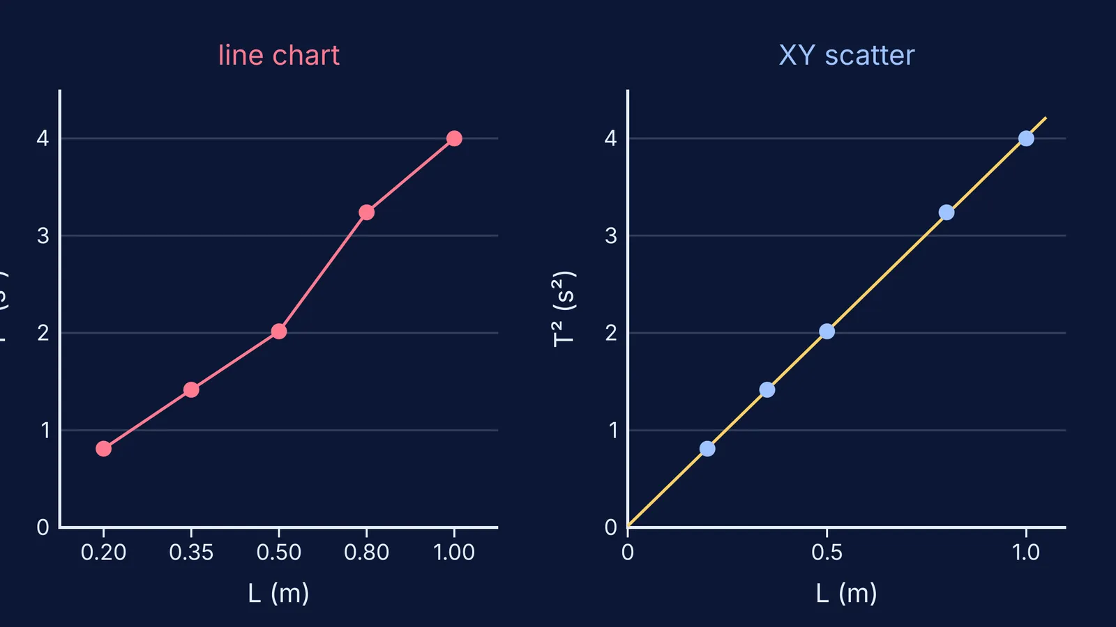
Before. Insert a line chart from the L and T² columns. The five lengths sit at equal gaps, and T² rises by 0.61, 0.60, 1.22, then 0.76, so a kink appears at 0.80 m. Nothing happened there: the 0.50 m to 0.80 m jump was squeezed into the same width as every other gap. No units, and a legend reading "Series1".
After.
Select the L and T² columns and insert a scatter chart with markers only.
Add axis titles: "L (m)" and "T² (s²)".
Add a linear trendline and tick "show equation" and "show R²".
Read the fit. With these readings, least squares gives a slope of 4.00 s²/m, an intercept under 0.02 s² and R² above 0.999.
Work out g = 4π²/slope = 39.48/4.00 ≈ 9.87 m/s², then compare it with the accepted value and discuss the gap.
The points now fall on one straight line that nearly passes through the origin, as the theory predicts.
For the full experiment, see our walk-through of measuring g with the L–T² graph method, and for what slopes and areas mean, reading physics graphs. If you want a feel for how a quantity responds before you take readings, the Fermi Simulation Lab has interactive simulations for ideas that are easier to see than to read.


