On this page
A treatment can win in every group of patients and still lose overall. That sounds like an arithmetic mistake, but it is a well-known pattern called Simpson's paradox. Once you see how it works, you can spot it in exam results and news headlines.
What is Simpson's paradox?
The Stanford Encyclopedia of Philosophy defines Simpson's paradox as a statistical phenomenon where an association between two variables in a population emerges, disappears or reverses when the population is divided into subpopulations.
It is named after Edward Simpson's 1951 paper on contingency tables, though the same entry notes that Karl Pearson (1899) and George Udny Yule (1903) described the effect earlier.
What is a real example of Simpson's paradox?
A widely taught example comes from a 1986 BMJ study by Charig and colleagues comparing ways of treating kidney stones; a 1994 BMJ note by Julious and Mullee later used it to explain confounding. Call the two treatments A (open surgery) and B (percutaneous nephrolithotomy, a keyhole method). The counts below are as tabulated in this statistics textbook chapter.
Read the two group results, then predict before you scroll.
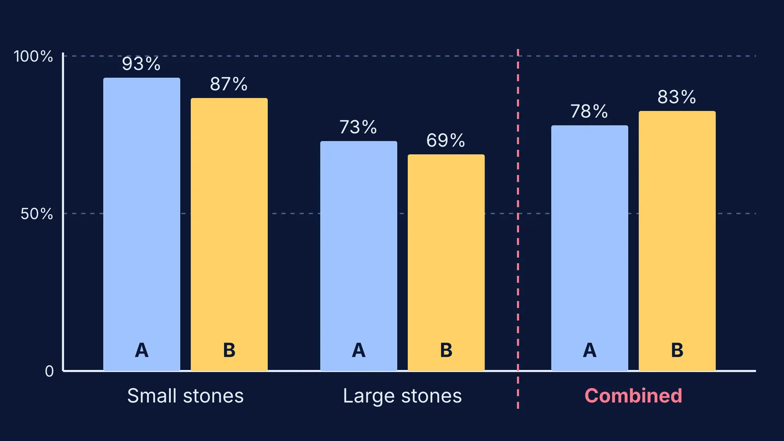
Small stones: A succeeded in 81 of 87 patients (93%), B in 234 of 270 (87%).
Large stones: A succeeded in 192 of 263 (73%), B in 55 of 80 (69%).
A wins for small stones and wins for large stones. So which treatment wins when you add the rows together?
All patients: A succeeded in 273 of 350 (78%), B in 289 of 350 (83%).
B wins overall. Nothing was miscounted: 81 + 192 = 273 and 234 + 55 = 289.
Why does the trend flip when you add the groups?
Look at who got each treatment. Of A's 350 patients, 263 had large stones, about 75%. Of B's 350 patients, only 80 had large stones, about 23% (counts from the textbook table).
Large stones are harder to treat with either method. So A's overall rate is mostly an average of hard cases, while B's is mostly an average of easy cases. The combined percentage is a weighted average, and the weights were very different for the two treatments.
Stone size here is a confounder: something linked both to which treatment a patient got and to whether it worked. Ignore it, and you end up comparing the mix of patients, not the treatments.
If weighted averages feel slippery, the same trap shows up in physics: our post on why average speed is not the average of the speeds uses the same idea, with time as the weight.
Try it yourself: can you predict the combined result?
Here is a made-up example for practice, with the same structure as the kidney-stone table in Dunn's textbook chapter. Riya and Kabir each attempt 100 practice questions before a JEE Main mock.
Easy questions: Riya gets 18 of 20 right (90%). Kabir gets 68 of 80 right (85%).
Hard questions: Riya gets 24 of 80 right (30%). Kabir gets 5 of 20 right (25%).
Riya is more accurate on easy questions and on hard ones. Now predict: who has the higher overall accuracy?
Work it out on paper. Riya: 18 + 24 = 42 of 100, so 42%. Kabir: 68 + 5 = 73 of 100, so 73%.
Kabir looks far better on the scoreboard only because he chose mostly easy questions.
Now change one thing and predict again. Give both students 50 easy and 50 hard questions at the same rates. Riya gets 45 + 15 = 60 right; Kabir gets 42.5 + 12.5 = 55. With the same mix, the flip disappears.
How do you spot Simpson's paradox in your own data?
Run through this checklist whenever you compare two combined percentages:
Split the total into its natural groups (difficulty, chapter, department, age).
Compare the rates inside each group, not just overall.
Check the group sizes on each side. Very different mixes are a warning sign.
Ask what decided who landed in which group. That is where the confounder hides.
Report both the group rates and the overall rate, and say which question each one answers.
The Berkeley admissions case is a related example. A 1975 Science paper by Bickel, Hammel and O'Connell found that aggregate figures for fall 1973 showed a clear but misleading pattern of bias against women. Few departments showed a significant bias either way, and when the department-level data were pooled properly, there was a small but statistically significant bias in favour of women. Women had tended to apply to departments that were harder to enter for applicants of either sex.
When you read percentages in the news, it also helps to keep percentage points and percent change apart, and to know what accuracy, precision and recall each measure.
If you like to change inputs and watch results move, the Fermi Simulation Lab has interactive simulations for ideas you need to see, not just read about. For this paradox, a pencil and the Riya and Kabir numbers are enough.