On this page
Before integration is a list of formulas, it is a picture: thin rectangles packed under a curve. Two questions make the picture useful. Is my stack of rectangles too tall or too short, and how quickly does it approach the true area? You can answer both before calculating anything.
What is a Riemann sum?
A Riemann sum approximates the area under y = f(x) on [a, b] by cutting the interval into n strips of width Δx = (b − a)/n and adding up f(x*)Δx, where x* is any point in each strip (OpenStax Calculus Volume 1, section 5.1). It is named after the 19th-century mathematician Bernhard Riemann, who developed the idea, as the same OpenStax section notes.
The two simplest choices are:
Left sum L_n: each rectangle's height is f at the left edge of its strip.
Right sum R_n: each rectangle's height is f at the right edge.
OpenStax defines the exact area under the curve as the limit of these sums as n goes to infinity.
When do left and right sums overestimate or underestimate?
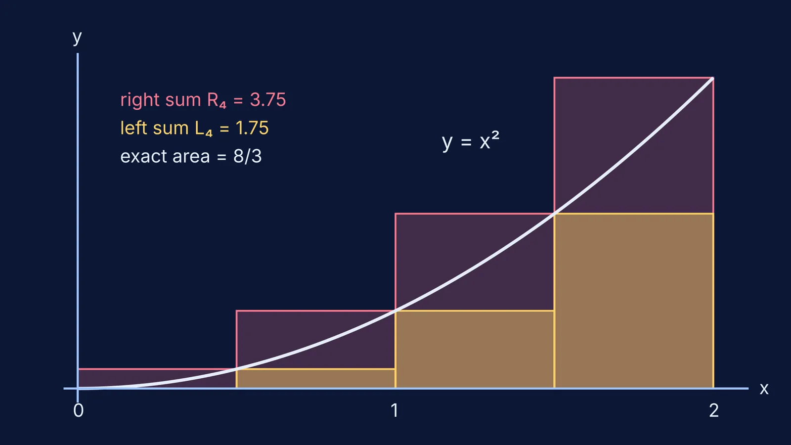
The left Riemann sum underestimates the area when f is increasing and overestimates it when f is decreasing; the right sum does the opposite (Riemann sum, Wikipedia).
The reason is visible in one rectangle. If the curve rises across a strip, its left edge is the lowest point, so a left rectangle sits entirely under the curve, while a right rectangle pokes above it.
The rule fails once the curve turns. Try y = sin x on [0, π] with four strips. Because sin 0 = sin π = 0, the left and right sums are the same number: (π/4)(0 + 0.7071 + 1 + 0.7071) ≈ 1.896, while the true area is 2. Both underestimate, because the curve bends downward and the gaps lose more than the overhangs gain.
A worked example: y = x² on [0, 2]
OpenStax works this case with four strips (Δx = 0.5) and gets L_4 = 1.75 and R_4 = 3.75 (OpenStax 5.1). The exact area is 8/3 ≈ 2.667, so the increasing-function rule holds: left is low, right is high.
Using the formula for the sum of squares, you can write both sums for any n:
L_n = 8/3 − 4/n + 4/(3n²)
R_n = 8/3 + 4/n + 4/(3n²)
Watch the errors:
n = 4: L = 1.750, R = 3.750, left error about 0.917
n = 8: L = 2.188, R = 3.188, left error about 0.479
n = 16: L = 2.422, R = 2.922, left error about 0.245
n = 32: L = 2.543, R = 2.793, left error about 0.124
Each doubling of n roughly halves the error. Notice also that R_n − L_n = 8/n every time. That is no accident: the two sums share every rectangle except the first left one and the last right one, so the gap is always (f(b) − f(a))Δx.
How fast do Riemann sums approach the integral?
For left and right sums, the error is at most M₁(b − a)²/(2n), where M₁ is the largest value of |f′(x)| on the interval (Wikipedia). The 1/n is why convergence feels slow: ten times the rectangles buys about one more correct decimal place.
The midpoint rule does much better. Its error is at most M(b − a)³/(24n²), with M the largest value of |f″(x)|, and the trapezoidal rule is exactly the average of the left and right sums, T_n = ½(L_n + R_n) (OpenStax Calculus Volume 2, section 3.6). For y = x², the midpoint sum with four strips is 2.625, already within 0.042 of 8/3, and doubling n cuts that error to a quarter.
How to practise Riemann sums on an interactive graph
A slider only teaches if you commit to an answer first. Parents can help by asking just one thing before each click: too big or too small? Use this routine:
Pick a function and interval. Say out loud whether it rises, falls or turns.
Before showing rectangles, predict: will the left sum be too big or too small? The right sum?
Set n = 4 and check. If you were wrong, find the one rectangle that proves it.
Predict the error at n = 8. For left or right sums, expect about half; for midpoint, about a quarter.
Change to a curve that turns, such as sin x on [0, π], and predict again.
The Fermi Simulation Lab has interactive simulations for ideas that are easier to see than to read, so you can run this routine instead of imagining the rectangles. If a textbook sum still will not come out right, the Fermi Problem Library has worked problems with a step-by-step solver that explains the reasoning rather than printing an answer.
Once over- and underestimates feel obvious, the next step is seeing why the area function's slope is the curve itself: see how the fundamental theorem connects area and derivatives, and pair it with the derivative as the slope of a tangent.