

On this page
When students first encounter definite integrals, they often view them as static numerical areas or mechanical antidifferentiation exercises. In Class 12 CBSE mathematics and entrance preparation like JEE, the syllabus formally separates integration into two theorems. The First Fundamental Theorem of Integral Calculus introduces the area function A(x) = ∫_a^x f(t) dt and asserts that its derivative is simply f(x). Yet, as mathematician David M. Bressoud pointed out in 2011, conventional classrooms rush straight to the Second Fundamental Theorem—evaluating ∫_a^b f(x) dx = F(b) − F(a)—leaving students without an intuitive picture of why differentiation and integration undo each other. Understanding accumulation as an active process provides the foundation for the calculus tools needed for mechanics and electromagnetism.
What is the area function in calculus?
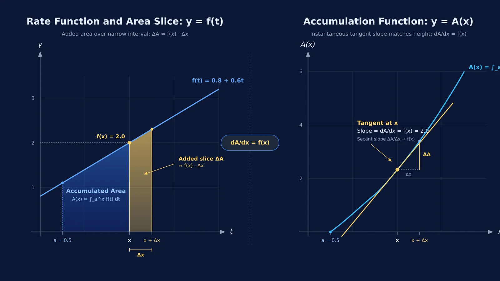
The area function A(x) tracks the accumulated signed area between a continuous curve y = f(t), the horizontal axis, and vertical boundaries from a fixed starting point t = a to a moving upper limit t = x:
A(x) = ∫_a^x f(t) dt
Notice the two distinct variables. The integration variable t acts as an internal dummy parameter sweeping from a to x, while x is the independent input that controls where accumulation stops.
At the starting boundary x = a, no area has accumulated, so A(a) = 0. As x advances to the right across positive regions of f(t), A(x) steadily grows. When f(t) dips below the horizontal axis, the integral accumulates negative signed area, reducing A(x). Rather than a single fixed number, the area function is a dynamic running total that changes continuously as the upper endpoint moves.
Why is the derivative of the area function equal to f(x)?
To see why A′(x) = f(x), consider what happens when you advance the right endpoint by a tiny increment Δx. The extra area added to your running total is:
ΔA = A(x + Δx) − A(x) = ∫_x^{x + Δx} f(t) dt
When Δx is narrow, the height of a continuous curve across that sliver barely changes. The newly added region is approximately a thin rectangular strip with width Δx and height f(x), giving an area of ΔA ≈ f(x) · Δx. Dividing by the step width Δx yields the average rate of area growth over that interval:
ΔA / Δx ≈ f(x)
Taking the limit as Δx approaches zero converts this difference quotient into an exact instantaneous derivative:
dA/dx = lim_{Δx → 0} (ΔA / Δx) = f(x)
This is the First Fundamental Theorem of Calculus. In his 1994 study in Educational Studies in Mathematics, Patrick W. Thompson observed that students who view rate solely as a static ratio struggle to grasp this result. Grasping the theorem requires seeing that the instantaneous rate at which a quantity accumulates is determined by the value of the rate function at that very instant.
How does dragging an endpoint build covariational reasoning?
Connecting curve height to the slope of accumulated area requires covariational reasoning—the cognitive ability to coordinate continuous changes in one variable with simultaneous changes in another. In a 2002 paper in the Journal for Research in Mathematics Education, Marilyn Carlson and colleagues showed that reaching Level 5 covariation—reasoning about instantaneous rates of change—is essential for calculus students to avoid common misconceptions. Without this mental model, learners often assume that when f(x) decreases, A(x) must decrease too, failing to realise that accumulation continues to grow as long as f(x) remains positive.
Dynamic environments make this relationship concrete. In a high school intervention, Anatoli Kouropatov and Tommy Dreyfus (2014) found that letting students drag an upper limit and watch accumulation in real time enabled them to construct the concept of the definite integral before memorising symbolic algorithms. Seeing a visual display transform as you drag reinforces how interactive simulations compare with static diagrams.
When dynamic ideas like accumulation feel abstract on paper, interactive tools help you test your intuition before running the algebra. The Fermi Simulation Lab provides interactive simulations for ideas that are easier to see than to read, letting you drag curve boundaries in real time to observe how the accumulated area traces out its derivative.
A five-step routine to predict and check the area function
To build a reliable intuition for accumulation problems, use this five-step prediction routine whenever you encounter an area function like A(x) = ∫_0^x 2t dt:
Locate the baseline zero: Identify where accumulation begins. Because the lower limit is 0, A(0) = 0.
Predict the sign of the slope: Look at the sign of f(t). Because f(t) = 2t is positive for all t > 0, every added strip is positive, so A(x) must strictly increase. At t = 0, f(0) = 0, meaning the graph of A(x) starts with a horizontal tangent.
Predict the curvature: Observe whether f(t) is rising or falling. Because f(t) = 2t increases with a constant slope of 2, each incoming strip is taller than the last. Accumulation accelerates, so A(x) must be concave upward.
Calculate the moving strip at a sample point: At x = 3, curve height is f(3) = 6. A tiny step of Δx = 0.01 adds an area of ΔA ≈ 6 × 0.01 = 0.06, confirming the instantaneous slope at x = 3 is exactly 6.
Integrate and differentiate to verify: Evaluate the integral symbolically: A(x) = [t²]_0^x = x². Differentiating yields A′(x) = d/dx (x²) = 2x, which matches f(x) identically.
How do area functions appear in exam problem-solving?
In Class 12 CBSE board exams and JEE Advanced, examiners frequently test whether students understand the area function by defining new functions through integrals with variable limits.
A classic exam question asks for the derivative of an accumulation function whose upper limit is itself a function of x, such as g(x) = ∫_0^{x²} sin(t²) dt. By applying the chain rule to the First Fundamental Theorem (the Leibniz rule), you differentiate directly with respect to the boundary:
g′(x) = sin((x²)²) · d/dx (x²) = 2x sin(x⁴)
Recognising the area function also prevents careless errors when finding stationary points and points of inflection. If g(x) is defined as an integral of f(t), then g′(x) = 0 occurs wherever the graph of f crosses the horizontal axis. Knowing how to relate the properties of an integrand to its integral avoids the traps detailed in interpreting slopes and areas on graphs.
Once you master the geometric intuition, tackling multi-step exam questions with variable limits becomes straightforward. The Fermi Problem Library provides worked problems with a step-by-step solver that explains the reasoning rather than printing an answer.


