

On this page
Push a child on a swing at the wrong moments and very little happens. Push in time with the swing and every push adds to the last. That is resonance, and a simulation is one of the clearest ways to watch it happen. You change the driving frequency, keep everything else the same, and watch the amplitude rise, peak and fall away.
Here is what to predict before you press play, and what real bridge failures do and do not tell you.
Where does the amplitude peak when you drive an oscillator?
Take a mass m on a spring of stiffness k, slowed by a damping force with constant b and pushed by a force F₀cos(ωt). After the start-up wobbles die away, the mass settles into steady oscillation at the driving frequency ω, not at its own frequency. Its amplitude is A = F₀ / √(m²(ω² − ω₀²)² + b²ω²), as derived in OpenStax University Physics, section 15.6.
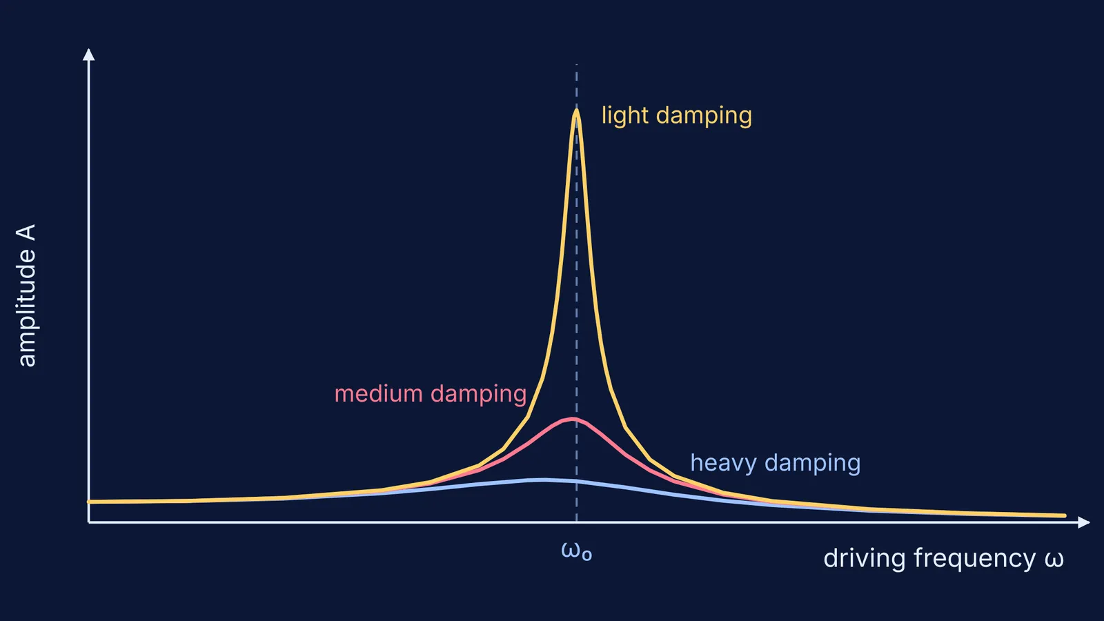
The natural frequency ω₀ = √(k/m) is the frequency at which the system would oscillate with no driving and no damping, in the OpenStax definition. Look at the formula: when ω equals ω₀, the first term under the root vanishes and only damping limits the amplitude. That is why the peak sits at, or very close to, ω₀.
The formula also gives you the two ends of the graph. Drive very slowly and the amplitude approaches F₀/k, the stretch a steady push would give. Drive very fast and the mass cannot keep up, so the amplitude falls towards zero.
How does damping change the resonance graph?
Damping does three things you can see in a simulation:
It lowers the peak. At resonance the amplitude is about F₀/(bω₀), and "the highest peak, or greatest response, is for the least amount of damping" (OpenStax).
It widens the peak. In the same chapter, the less the damping, the narrower the resonance.
It nudges the peak to a slightly lower frequency. Set the derivative of A to zero and you find the peak at √(ω₀² − b²/(2m²)), a shift you will only notice with heavy damping.
The sharpness has a name: the quality factor Q = ω₀/Δω, which for light damping is about mω₀/b (OpenStax). The same idea appears in AC circuits, which we cover in LCR resonance: quality factor, bandwidth and power factor.
A simulation run: predict, then check
Set up m = 1 kg, k = 100 N/m and F₀ = 1 N. Then ω₀ = 10 rad/s, about 1.6 Hz. Every number below comes from the OpenStax amplitude formula.
Drive at 1 rad/s with any damping. Predict about 1 cm, the static stretch F₀/k.
Set b = 0.5 kg/s and drive at 10 rad/s. Predict F₀/(bω₀) = 20 cm, twenty times the static stretch, with Q = 20.
Raise b to 2 kg/s, still at 10 rad/s. Predict 5 cm and Q = 5: a quarter of the height, much wider.
Raise b to 5 kg/s. The peak drops to about 2.1 cm and moves down to about 9.35 rad/s.
Drive at 20 rad/s. The three settings give between about 0.32 and 0.33 cm, because far from resonance the spring and the mass's inertia matter more than the damping.
If your screen disagrees with a prediction, check whether you waited for the start-up wobbles to settle. For more practice at predicting first, see our guide to learning waves with simulations.
Why can bridges and glasses fail at resonance?
A lightly damped object has a tall, narrow peak, so a small, steady push at exactly the right frequency builds a large motion. OpenStax asks readers to explain, in terms of resonance, the trick of a performer singing a note toward a crystal glass until it shatters (source). Glass has little damping, so its peak is narrow and the singer has to match its natural frequency closely.
London's Millennium Footbridge opened on 10 June 2000 and was ordered closed on 12 June after footfalls set the deck swaying sideways at 0.5 to 1.1 Hz, with accelerations up to 0.25 g, according to Douglas Taylor's case study of the retrofit. The fix was the one your simulation suggests: add damping. Engineers fitted fluid dampers and tested the bridge with groups of up to 2,000 people.
The Tacoma Narrows Bridge of 1940 is the famous case, but it is not simple forced resonance. Billah and Scanlan, in the American Journal of Physics (1991), argued that the failure came from aerodynamic self-excitation, or "negative damping", in a twisting motion. They also stated that forced resonance and self-excitation are fundamentally different.
How do you get the most from a resonance simulation?
Change one thing per run: frequency first, then damping.
Predict the peak frequency and height before each run, then compare.
Sketch amplitude against frequency yourself from five or six runs.
Ask why the far-off-resonance values barely move when you change damping.
For what studies have found about learning this way, read what PhET research says interactive simulations are good for. To run the experiment yourself, the Fermi Simulation Lab has interactive simulations for ideas that are easier to see than to read. If the formula is the sticking point, the Fermi Concept Library gives each concept its own lesson.


