On this page
When rolling a standard six-sided die, landing a six can feel like a quick sprint or an endless drought. One player rolls a six on their first try, while another waits through round after round without seeing one. How many rolls should you expect on average?
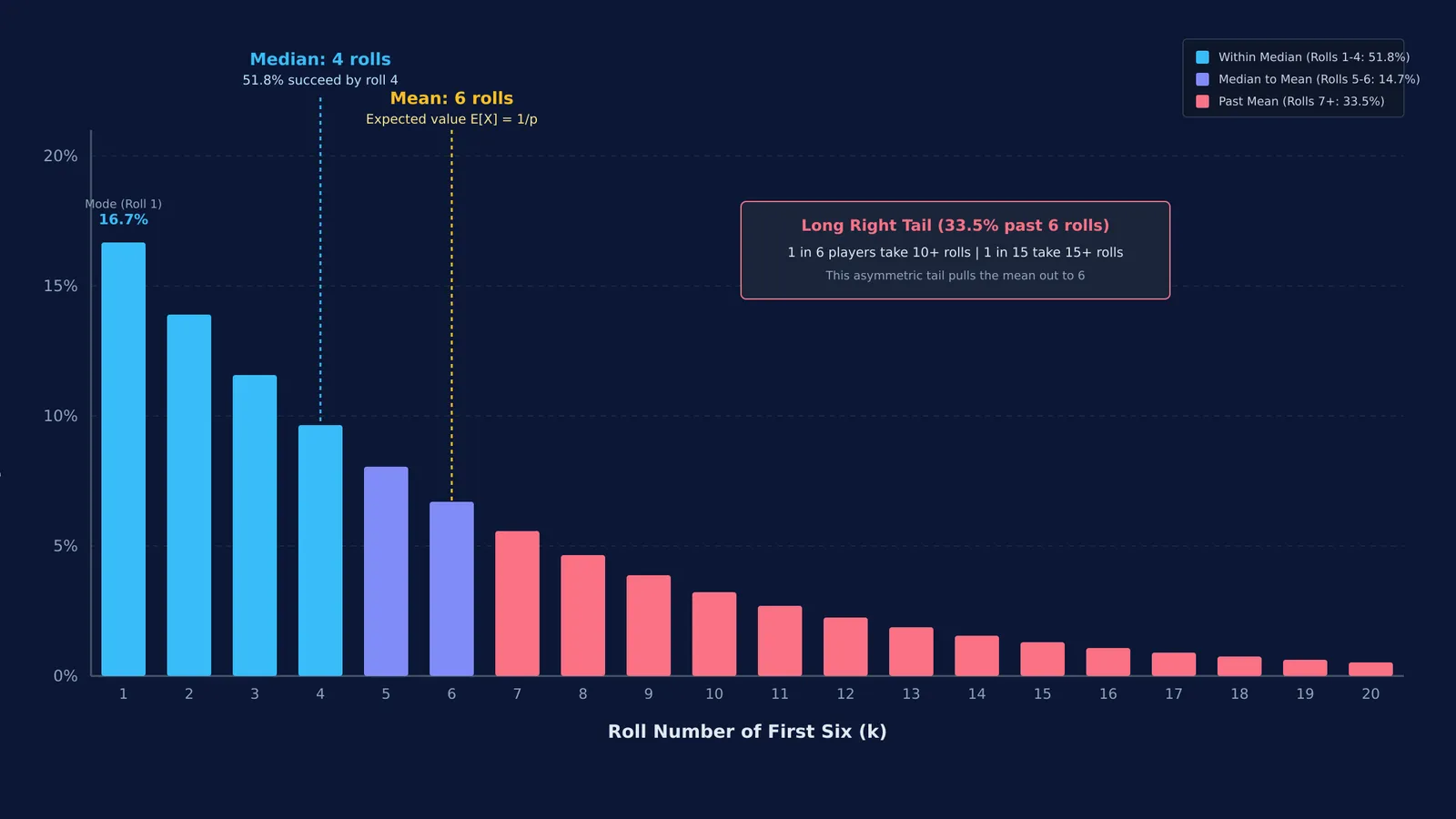
The mathematical answer is 6 rolls. Under the Wolfram MathWorld geometric distribution model, the expected trials until first success in an independent Bernoulli sequence with probability p is 1/p. Because each face has probability 1/6, the mean is 1 / (1/6) = 6. Yet this average hides a paradox: over 51% of players roll a six within 4 rolls, while a minority endures dry streaks.
What is the average number of rolls to get a six?
To understand this average, we define a discrete random variable X as the roll of the first six. Each roll is independent, with success probability p = 1/6 and failure probability q = 5/6. As outlined in OpenStax Introductory Statistics, the probability of the first six occurring on roll k is P(X = k) = (5/6)^(k−1) × (1/6).
First-step analysis gives the expected value E[X]: on roll 1, you roll a six with probability 1/6, ending the trial. With probability 5/6, you miss, using 1 roll and resetting the experiment to expect E[X] more rolls. This sets up E[X] = (1/6)(1) + (5/6)(1 + E[X]) = 1 + (5/6)E[X], which yields (1/6)E[X] = 1, or E[X] = 6. Summing the series ∑ k(5/6)^(k−1)(1/6) yields the same result, as detailed in our guide on probability distributions and random variables.
Why does the average take 6 rolls if the median is 4?
If the expected value is 6, why do typical players feel a six arrives faster? The reason lies in the distribution's skewness. As established in the Wolfram MathWorld geometric distribution model, the mode is 1. Roll 1 is the single most likely turn to produce a six, with a probability of 1/6 (approximately 16.67%). Each subsequent roll becomes less likely to host the first success because all prior rolls must fail first.
The median is the roll count where cumulative probability passes 50%:
Exactly 1 roll: 16.67%
Within 2 rolls: 1 − (5/6)² = 11/36 ≈ 30.56%
Within 3 rolls: 1 − (5/6)³ = 91/216 ≈ 42.13%
Within 4 rolls: 1 − (5/6)⁴ = 671/1296 ≈ 51.77%
Under the geometric distribution cumulative distribution function, over 51% of trials finish within 4 rolls. The median wait is therefore 4 rolls, not 6. The mean is pulled to 6 by the heavy right tail of unlucky runs, a dynamic we analyze in our article on probability in repeated trials.
How do you calculate the probability of a long dry streak?
The right-hand tail of the geometric distribution explains why players frequently experience agonizing waits. The probability of failing to roll a six in k consecutive attempts is P(X > k) = (5/6)^k.
Using formulas from OpenStax Introductory Statistics, tail probabilities show how common streaks are:
Failing for 6 rolls: (5/6)⁶ ≈ 33.49% (about 1 in 3 trials)
Failing for 10 rolls: (5/6)¹⁰ ≈ 16.15% (nearly 1 in 6 players)
Failing for 15 rolls: (5/6)¹⁵ ≈ 6.49% (about 1 in 15 players)
Failing for 20 rolls: (5/6)²⁰ ≈ 2.61% (about 1 in 38 players)
Failing for 30 rolls: (5/6)³⁰ ≈ 0.42% (about 1 in 237 players)
These numbers show that rolling 10 or 15 times without a six is ordinary variation. In a class of 40 students rolling dice simultaneously, probability models predict that several will endure dry streaks exceeding 10 rolls.
Why does a six feel overdue when you roll five misses?
When you roll five misses in a row, intuition often insists a six is "due," a cognitive distortion known as the gambler's fallacy. In their 1971 Psychological Bulletin paper, psychologists Amos Tversky and Daniel Kahneman documented the "belief in the law of small numbers," showing that people expect small samples to mirror population odds. In their 1974 Science study on heuristics and biases, they explained how the representativeness heuristic leads observers to view streaks as imbalances that chance must correct.
A die has no memory. As documented in OpenStax Introductory Statistics, the geometric distribution is memoryless: P(X = k + m | X > m) = P(X = k). After five misses, the chance of a six on the next roll remains 1/6 (approximately 16.67%), with past misses providing zero momentum. Review common traps in our guide to five common probability mistakes in JEE maths.
How can simulating thousands of dice rolls reveal the long tail?
Formulas provide exact values, but experimentation builds intuition. Under the law of large numbers, simulations show how random streaks assemble into a smooth theoretical distribution. You can test this in four steps:
Generate random integers from 1 to 6 until a 6 appears.
Record the roll count.
Repeat across 10,000 trials to calculate the mean and median.
Plot the frequencies as a histogram.
Across 10,000 trials, the average hovers near 6.0, but the histogram peaks at 1 and stretches past 25 rolls. The Fermi Simulation Lab provides interactive simulations for ideas that are easier to see than to read, helping students see how random streaks behave.
For students tackling problem sets on random variables, the Fermi Problem Library offers worked problems with a step-by-step solver that explains the reasoning rather than simply displaying a final number. Combining derivations with simulations ensures you never confuse an expected value with a guaranteed outcome.