
On this page
In the early 1910s, in Brno, Viktor Kaplan patented a water turbine that looks like a ship's propeller with one important difference: its blades can turn. That let engineers make electricity efficiently from wide rivers that fall only a few metres, even as the flow rises and falls.
Who was Viktor Kaplan?
Kaplan was born in Mürzzuschlag, Austria, on 27 November 1876 and died on 23 August 1934, according to the Austria-Forum biography. It records that he was a professor at the University of Technology in Brno from 1913 to 1932, and that after 1912 he designed “a new water turbine with variable pitch runner blades, which could also be used for low heads in river power stations”.
Brno University of Technology, whose fluid engineering department is now named after him, says he patented the design in 1913 and that it is “suitable for low gradients and high flows”. The Wikipedia article on the Kaplan turbine dates his first patent to 1912.
Early machines suffered from cavitation, where vapour bubbles collapse against the blades, and Kaplan abandoned his research in 1922 for health reasons, the same article says. By 1924 an 8 MW unit was running at Lilla Edet in Sweden.
Why do low-head rivers need a different turbine?
Head is the height the water falls. A hydro plant's power is P = ηρgQH, where ρ is water density (about 1000 kg/m³), g is 9.81 m/s², Q is the flow in cubic metres per second, H is the head in metres and η is the efficiency, typically 0.75 to 0.95 (Engineering ToolBox).
Take a river weir with a 10 m head, a flow of 100 m³/s and an efficiency of 0.9. P = 0.9 × 1000 × 9.81 × 100 × 10 ≈ 8.8 MW. A 500 m mountain head gets the same power from just 2 m³/s. The low-head plant must swallow 50 times more water, so it needs a wide opening with water flowing straight through, like air through a fan.
The US Department of Energy notes that Pelton wheels are used for very high heads and low flows, and Francis turbines for medium to high heads of 130 to 2,000 feet. You can read how Lester Pelton's split-cup wheel reverses the water's momentum and how James Francis built the turbine that powers India.
How do adjustable blades work in a Kaplan turbine?
Water enters through a ring of wicket gates, then flows along the axis through the runner. In a Kaplan turbine, “both the blades and the wicket gates are adjustable, allowing for a wider range of operation”, says the Department of Energy.
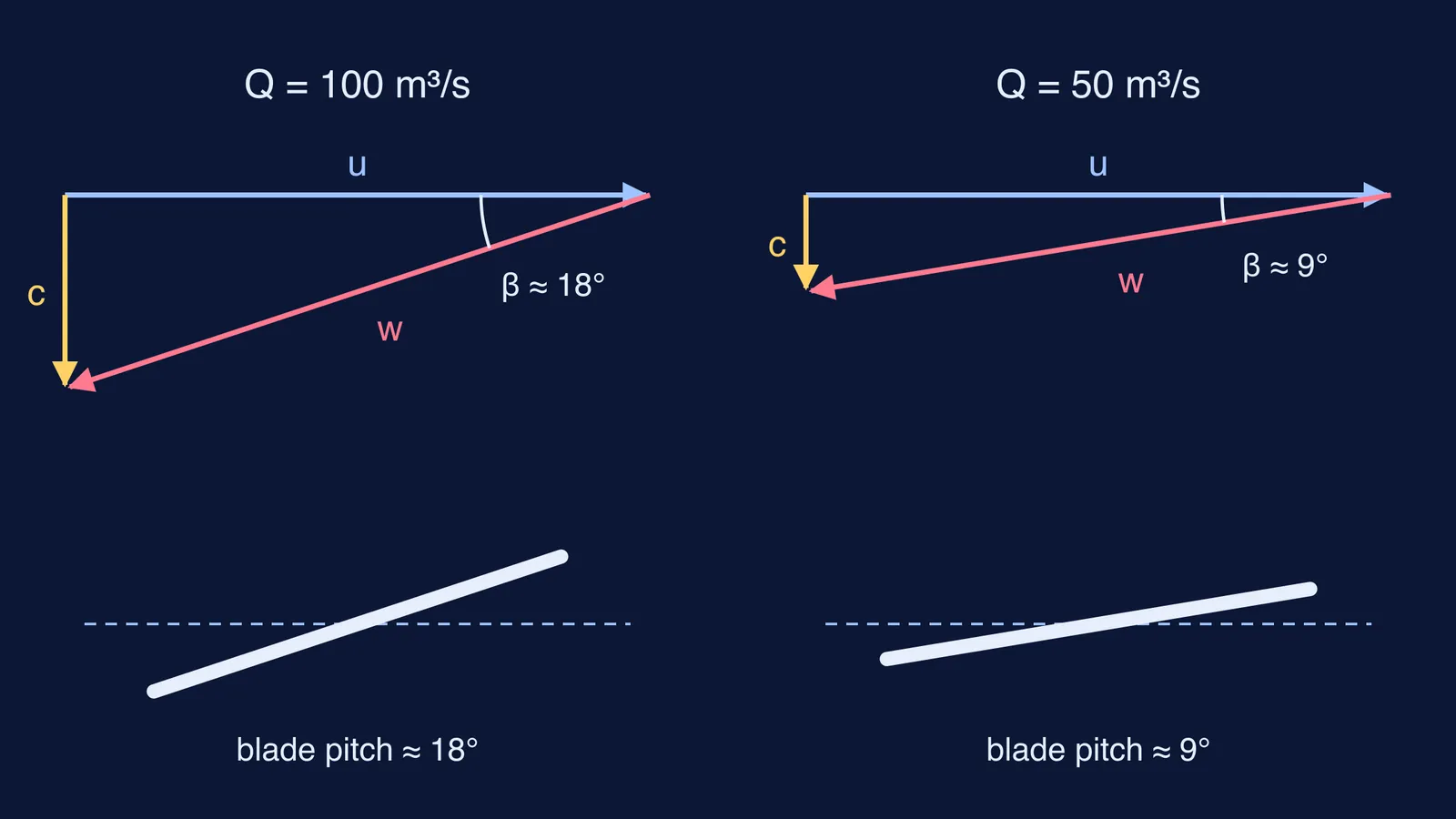
Why the angle matters comes down to a velocity triangle. Each slice of blade moves sideways at speed u = ωr. Water moves along the axis at c = Q/A, where A is the open ring between hub and tip. Seen from the moving blade, the water flows along a relative velocity w. If it leaves with no swirl, w makes an angle β to the plane of rotation, with tan β = c/u. Blades out of line with this flow waste energy churning water.
Worked example: one runner, two river flows
Runner diameter 5 m, hub 2 m, speed 100 rpm. Flow area A = π/4 × (5² − 2²) ≈ 16.5 m².
At the mean radius of 1.75 m, u = 2π × 100/60 × 1.75 ≈ 18.3 m/s.
Monsoon flow, Q = 100 m³/s: c ≈ 6.06 m/s, tan β ≈ 0.33, so β ≈ 18°.
Dry-season flow, Q = 50 m³/s: c ≈ 3.03 m/s, tan β ≈ 0.17, so β ≈ 9°.
Halving the flow halves c while u stays the same, so the best angle drops from about 18° to about 9°. Fixed blades would meet the dry-season water at the wrong angle; Kaplan's runner turns its blades flatter. Real blades are also twisted, because u grows towards the tip.
Where are Kaplan turbines used today?
Kaplan turbines typically work at heads of 10 to 70 m and produce 5 to 200 MW, according to the Kaplan turbine overview on Wikipedia. Their efficiency is typically over 90%, though lower at very low heads.
India has them too. NHPC's Tanakpur Power Station on the Sharda river in Uttarakhand, commissioned in 1992, runs three 40 MW Kaplan units at a net head of 24.3 m (Power Technology plant profile).
How can you practise this?
Find the flow. Assume η = 0.9 for one Tanakpur unit: Q = 40,000,000 ÷ (0.9 × 1000 × 9.81 × 24.3) ≈ 186 m³/s.
Compare a high head. The same 40 MW from a 500 m head needs only about 9 m³/s.
Draw two triangles. Sketch u, c and w for full and half flow and measure β with a protractor.
If the triangles are hard to picture, the Fermi Simulation Lab has interactive simulations for ideas that are easier to see than to read. If your numbers keep going wrong, the Fermi Problem Library has a step-by-step solver that explains the reasoning rather than printing an answer.