On this page
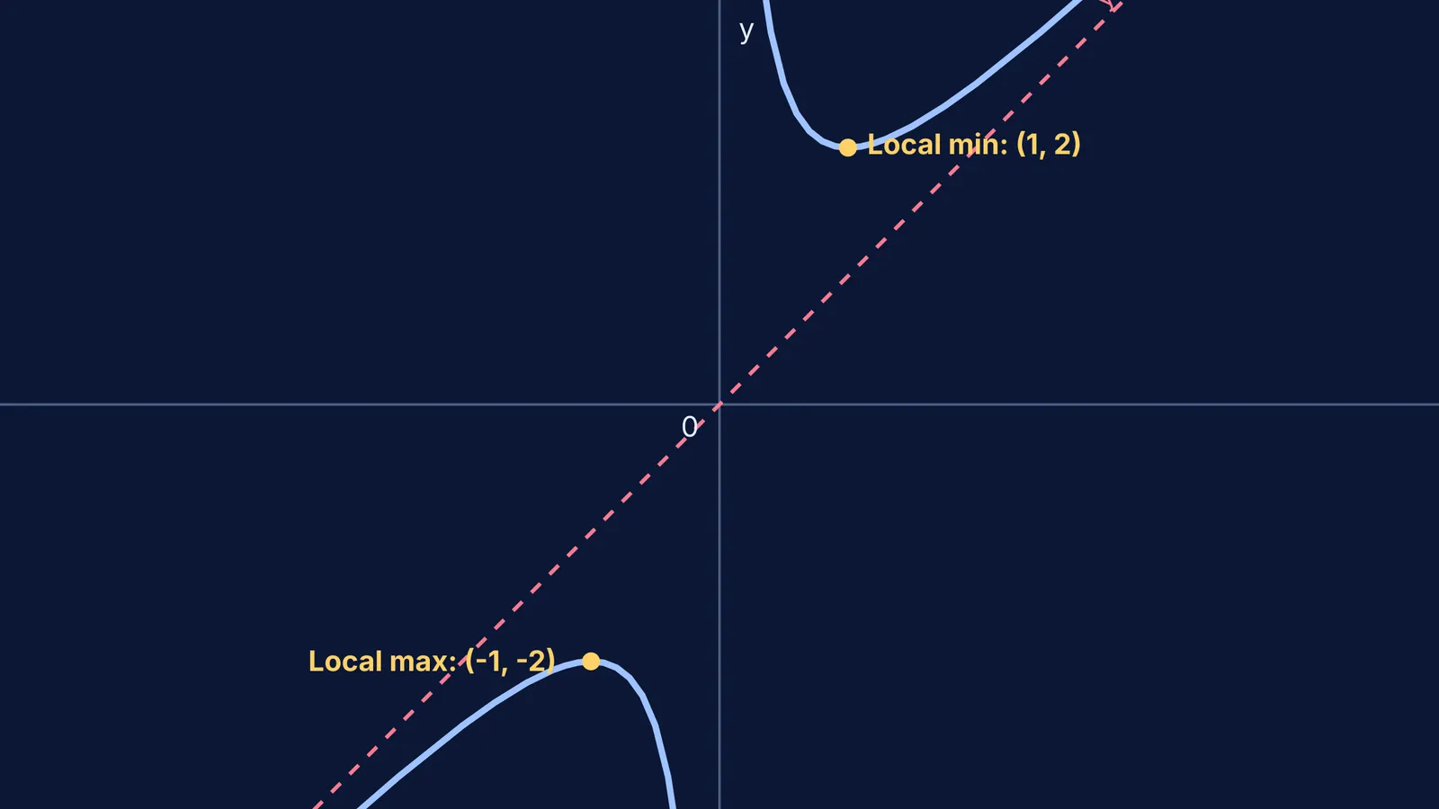
Most continuous curves go up to a maximum, turn around, and go down to a minimum. But rational functions can behave differently. When you sketch the curve y = x + 1/x, you find a strange result: its lowest turning point (local minimum) is physically higher on the y-axis than its highest turning point (local maximum).
According to the OpenStax textbook Calculus Volume 1 (OpenStax), the shape of a graph is determined by its asymptotes, its first derivative (which gives the turning points), and its second derivative (which gives the concavity). Here is how to apply those rules to y = x + 1/x.
What are the asymptotes of x + 1/x?
An asymptote is a line that a curve approaches as it heads towards infinity (OpenStax). This curve has two.
The vertical asymptote: The function y = x + 1/x is undefined at x = 0 because you cannot divide by zero. As x approaches zero from the positive side, the 1/x term grows infinitely large, so the curve shoots up towards +∞. As x approaches zero from the negative side, 1/x becomes a very large negative number, so the curve drops to -∞. This makes the y-axis (x = 0) a vertical asymptote.
The oblique asymptote: To see what happens at the far ends of the graph, look at the limit as x becomes very large. As x approaches +∞ or -∞, the 1/x fraction shrinks to zero. The function essentially becomes y = x + 0. This means the graph gets closer and closer to the diagonal line y = x. This is known as an oblique or slant asymptote.
How do you find the minimum and maximum of y = x + 1/x?
To find the turning points, we use the first derivative test. The first derivative tells us the slope of the curve.
Differentiate f(x) = x + x⁻¹ to get f′(x) = 1 - 1/x².
Set the derivative to zero to find the critical points: 1 - 1/x² = 0, which means x² = 1. The solutions are x = 1 and x = -1.
Calculate the y-coordinates. When x = 1, y = 1 + 1 = 2. When x = -1, y = -1 - 1 = -2.
To check which is a minimum and which is a maximum, we look at the second derivative, f″(x) = 2/x³.
At x = 1, the second derivative is positive (2). A positive second derivative means the curve is concave up (shaped like a smile), so (1, 2) is a local minimum.
At x = -1, the second derivative is negative (-2). A negative second derivative means the curve is concave down (shaped like a frown), so (-1, -2) is a local maximum.
Another important property of this function is its symmetry. If you replace x with -x, you get f(-x) = -x + 1/(-x) = -(x + 1/x) = -f(x). A function that satisfies f(-x) = -f(x) is called an odd function. This means the graph has rotational symmetry about the origin (0, 0). If you take the right-hand branch and rotate it 180 degrees around the origin, it maps perfectly onto the left-hand branch. This explains why the local maximum at (-1, -2) is an exact, upside-down reflection of the local minimum at (1, 2).
Why is the local minimum greater than the local maximum?
It seems contradictory for a minimum to be 2 while a maximum is -2. This happens because the graph is broken into two separate branches by the vertical asymptote at x = 0.
The point (1, 2) is a local minimum. It is the lowest point on the right-hand branch of the curve (where x > 0), but it is not the lowest point of the whole function. Similarly, (-1, -2) is the highest point on the left-hand branch (where x < 0). Because the two branches never connect, the function never crosses the space between y = -2 and y = 2. The range of the function is (-∞, -2] ∪ [2, ∞).
How can you check your curve-sketching working?
When solving curve-sketching problems, it is easy to make a sign error in the derivative and flip the minimum and maximum. A good habit is to test a value on either side of your critical point. For example, if you think (1, 2) is a minimum, test x = 0.5 and x = 2:
At x = 0.5, y = 0.5 + 2 = 2.5.
At x = 2, y = 2 + 0.5 = 2.5.
Both values are greater than 2, confirming that y = 2 is indeed the lowest point in that region.
You can also use this point-testing method to verify the concavity. Between x = 0 and x = 1, the curve must drop from infinity down to the minimum at (1, 2). From x = 1 onwards, the curve rises again, getting closer and closer to the line y = x. This continuous cup shape confirms the positive second derivative. On the left side, the curve rises from -∞ along the line y = x, hits a peak at (-1, -2), and then plunges down to -∞ as it approaches the y-axis, creating an upside-down cup that matches the negative second derivative.
If you are stuck on the calculus, the Fermi Problem Library has worked problems with a step-by-step solver that explains the reasoning rather than printing an answer. This helps you see how the first and second derivative tests apply to other rational functions.
For more practice with reading graphs, try to Sketch the graph before you plot it: six functions to test or review how to use the second derivative in Concavity and points of inflection: the f″ sign-change test.