On this page
You see an integral from 1/2 to 2, or from 0 to ∞, with ln x or tan⁻¹ x inside, and no antiderivative fits. Those limits are the signal to try x = 1/t. Here is why it works, a quick test, and four worked examples.
Why does x = 1/t work for limits 1/a to a?
The substitution x = 1/t sends 1/a to a and a to 1/a, so the interval lands on itself, backwards. The same happens on 0 to ∞.
Two rules from the NCERT Class 12 Mathematics chapter on integrals do the rest. Property P0 says the name of the variable does not matter: ∫ f(x) dx = ∫ f(t) dt over the same limits. Property P1 says that swapping the limits changes the sign (we unpack this in why swapping limits changes the sign of an integral). Section 7.9 of the same chapter adds that when you substitute in a definite integral, the limits change along with the variable.
Now put x = 1/t, so dx = −dt/t². The minus sign from dx cancels the minus sign from flipping the limits back, and you are left with:
∫ from 1/a to a of f(x) dx = ∫ from 1/a to a of g(t) dt, where g(t) = f(1/t)/t².
Everything depends on how g compares with f.
How do you know when to use x = 1/t?
Look for two signals together:
The limits multiply to 1 (1/2 and 2, 1/3 and 3, 1/e and e), or they are 0 and ∞.
The integrand is built from pieces that behave well under x → 1/x: ln x, tan⁻¹ x, x − 1/x, x + 1/x, 1 + x² or a power xⁿ.
Then work out g(t) = f(1/t)/t² and sort it into one of four cases:
g = −f. The integral equals its own negative, so I = 0.
g = f. A pure mirror: the piece from 1/a to 1 equals the piece from 1 to a, so I = 2 × (integral from 1 to a).
f + g is simple. Add the two versions: 2I = ∫ (f + g), then halve.
None of these. Put the substitution down and try another method.
Which integrals can x = 1/t solve?
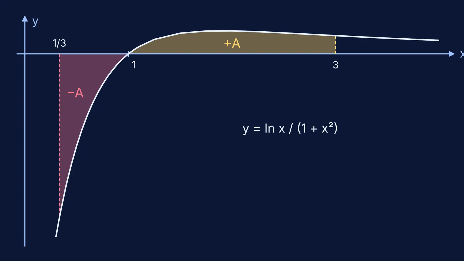
Example 1: ln x/(1 + x²) from 1/2 to 2. Here f(1/t) = (−ln t)/(1 + 1/t²) = −t² ln t/(1 + t²). Divide by t²: g(t) = −ln t/(1 + t²) = −f(t). That is case 1, so the integral is 0, as it is for 0 to ∞ or any 1/a to a. The graph at the top shows why: the deep, narrow area below the axis between 1/3 and 1 matches the long, shallow area above it between 1 and 3.
Example 2: sin(x − 1/x)/x from 1/2 to 2. Here f(1/t) = t·sin(1/t − t) = −t·sin(t − 1/t). Divide by t²: g(t) = −sin(t − 1/t)/t = −f(t). Case 1 again, so the answer is 0, because x − 1/x changes sign under x → 1/x.
Example 3: tan⁻¹ x / x from 1/2 to 2. Here f(1/t) = t·tan⁻¹(1/t), so g(t) = tan⁻¹(1/t)/t. For t > 0, tan⁻¹ t + tan⁻¹(1/t) = π/2, as these TU Delft calculus notes state. So f + g = (π/2)/t, which is case 3:
2I = (π/2) × [ln t] from 1/2 to 2 = (π/2)(2 ln 2), so I = (π/2) ln 2, about 1.09.
The same notes show the sum is −π/2 for negative t, so use this only when both limits are positive.
Example 4: 1/((1 + x²)(1 + xⁿ)) from 0 to ∞. Here g(t) = tⁿ/((1 + t²)(1 + tⁿ)), so f + g = 1/(1 + t²). Adding gives 2I = [tan⁻¹ t] from 0 to ∞ = π/2, so I = π/4 for every n. The value does not depend on n at all, which makes it worth recognising on sight.
The same adding idea drives the f(x) + f(1 − x) pairing trick for sums and integrals.
What mistakes should you check for?
Dropping the 1/t² factor that comes from dx.
Counting the minus sign twice, from dx and again after flipping the limits back.
Using x = 1/t on limits like 1 to 2, which become a different interval (1/2 to 1).
Using tan⁻¹(1/t) = π/2 − tan⁻¹ t when t can be negative.
You can also check a result; see how to check an integral by differentiating and testing limits.
If you keep getting stuck at the g(t) step, the Fermi Problem Library has worked problems with a step-by-step solver that explains the reasoning rather than printing an answer, so you can compare each step with your own working. If P0 and P1 still feel shaky, the Fermi Concept Library gives each mathematics concept its own lesson.
Next time you see limits that multiply to 1, spend thirty seconds on g(t) before anything else.