
On this page
Pull a bowstring back and you are doing work. The limbs bend, and that work sits in them as elastic potential energy until you let go. Then the limbs spring back, the string pushes the arrow, and most of the stored energy becomes the arrow's kinetic energy. It is the Class 11 work-energy chapter, in a form you can hold.
How does a bow store energy when you draw it?
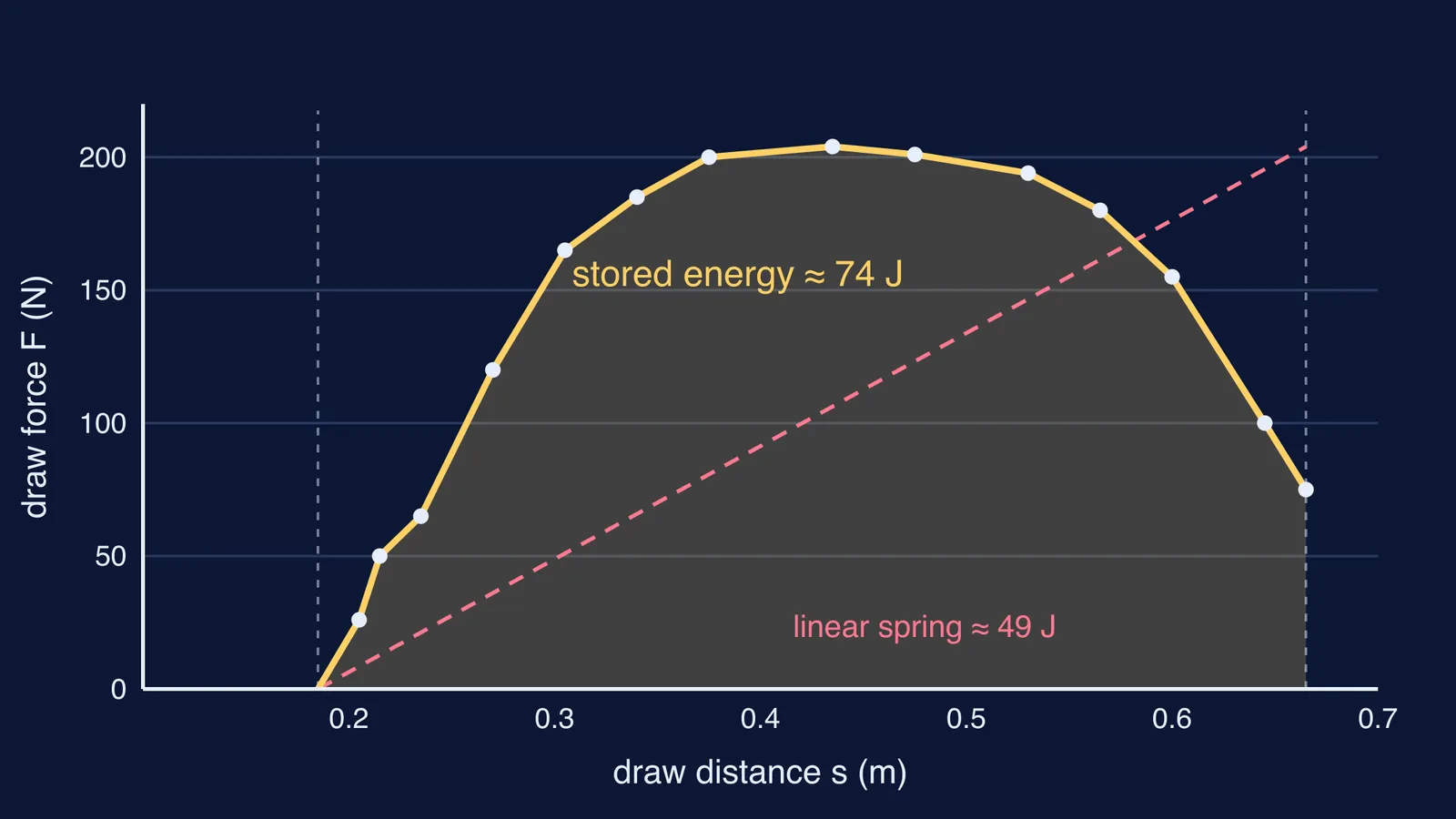
For an ideal spring, the stored elastic potential energy is U = ½kx², as OpenStax University Physics, section 8.1 sets out. A bow's limbs act like a stiff, bent spring, but their force does not rise in a neat straight line. So the useful rule is the general one: the work done by a varying force is the area under its force-displacement graph (OpenStax, section 7.1).
Archers call this graph the force-draw curve: the pull on the string at each point of the draw. Physicist H. O. Meyer of Indiana University measured it carefully for a compound bow in his paper Applications of Physics to Archery. The string rested 0.185 m from the grip (the brace height) and was drawn a further 0.481 m. Integrating the measured curve, Meyer found that drawing the bow put 73.7 J of work into it.
For the straight-line spring version of this graph, see our Hooke's law spring extension simulation.
Where does the energy go when you release the string?
Not all of it reaches the arrow. Meyer also measured the force while letting the string back slowly, and the energy available for the shot came out at 71.0 J, 3 to 4% less than went in, lost to internal friction in the limbs and friction in the cams (Meyer, arXiv:1511.02250). He notes that for old wooden bows, frictional losses of up to 20% were reported.
The arrow, with a mass of 20.6 g, left the bow with 57.1 J of kinetic energy. The gap is mostly because the string and limbs are still moving when the arrow separates, so they carry kinetic energy too. Meyer uses Klopsteg's idea of a "virtual mass" m̃ for the bow's moving parts: about 5 g. The efficiency, arrow energy divided by available energy, is then ε = M/(M + m̃), which is 0.80 for his bow.
The friction loss is the same idea as elastic hysteresis in rubber: the unloading curve sits below the loading curve.
How fast does the arrow leave the bow?
Use Meyer's numbers from his archery paper and the work-energy theorem, which says the net work done equals the change in kinetic energy (OpenStax, section 7.3).
Energy available for the shot: W = 71.0 J.
It is shared between the arrow (M = 0.0206 kg) and the bow's virtual mass (m̃ ≈ 0.005 kg), both moving at the launch speed v, so W = ½(M + m̃)v².
Solve: v = √(2W/(M + m̃)) = √(142/0.0256) ≈ 74.5 m/s.
Check: the arrow's energy is ½ × 0.0206 × 74.5² ≈ 57 J, matching the measured 57.1 J.
Now swap in a heavier 25 g arrow. The speed becomes √(142/0.030) ≈ 69 m/s, slower, but the efficiency rises to 25/30 ≈ 83%. Meyer's chronograph readings for three arrows show the same trend.
For the rubber-band version of this reasoning, see what happens when you stretch a rubber band twice as far.
Why does the shape of the force-draw curve matter?
In Meyer's data, the compound bow's draw force rises steeply to about 200 N, stays near it over much of the draw, and then drops sharply near full draw; he puts this "let-off" at about 65%. Now imagine a simple spring that rose in a straight line to the same peak of about 204 N (the highest point on his graph) over the same 0.48 m. Its area would be a triangle: ½ × 204 × 0.48 ≈ 49 J. The real bow stores about 74 J for the same peak pull, roughly half as much again, because its curve stays high for longer.
How do you solve a bow-and-arrow energy problem?
Run this checklist on any board or JEE Main question about bows, catapults or spring guns:
Name the store: the energy sits in the bent limbs as elastic potential energy, not in the arrow.
If the force is linear (F = kx), use U = ½kx². If you are given a graph, use the area under it.
Subtract losses only if the question gives an efficiency or a loss.
Set the energy that reaches the arrow equal to ½mv² and solve for v.
Sanity-check: a heavier arrow should come out slower.
If areas under curves still feel abstract, the Fermi Simulation Lab has interactive simulations for ideas that are easier to see than to read. When you set up a problem and get stuck on the method, the Fermi Problem Library has worked problems with a step-by-step solver that explains the reasoning rather than printing an answer.