On this page
What is the most common mistake with physics graphs?
When you see a position-time graph with a curved line, it is tempting to imagine a ball flying through the air in exactly that shape. This is the most common trap in kinematics. A 1994 study of 895 high school and college students published in the *American Journal of Physics* found that a large number of students misinterpret graphs as literal pictures of the motion (Beichner, 1994).
A graph is not a map of the physical world. A straight line on a graph can represent an object moving in a circle, and a curved line can represent an object moving in a perfectly straight line. The shape of the line on the paper tells you how a specific quantity—such as velocity—changes as time passes, not where the object is in space.
What do the slope and area of a graph mean?
Every line on a physics graph holds hidden information in its gradient (slope) and the two-dimensional space underneath it (area). The trick is knowing which one gives you the answer you need.
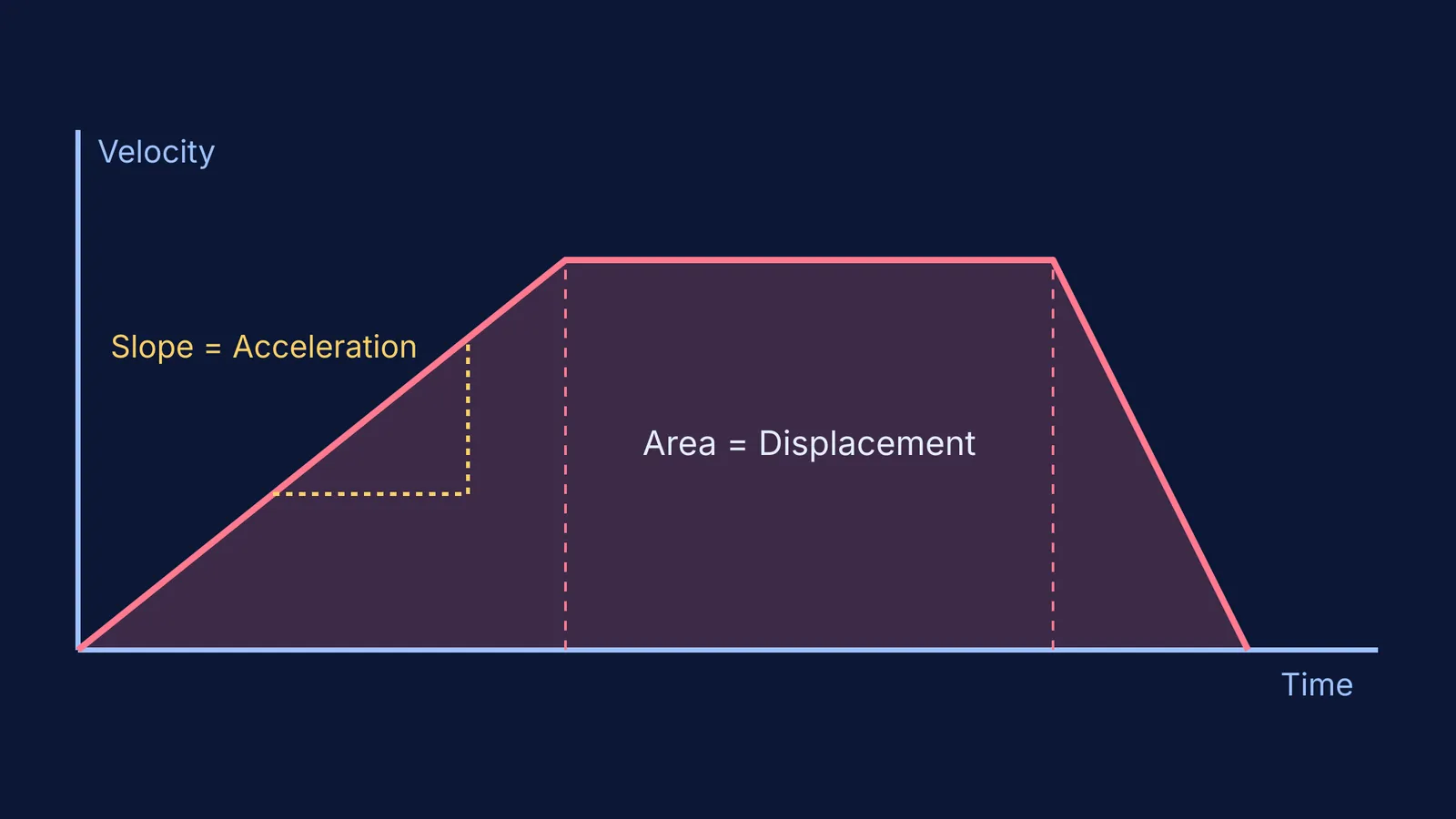
Slope: The slope is the "rise over run", which means the change in the y-axis divided by the change in the x-axis (Δy / Δx). If the y-axis is velocity and the x-axis is time, the slope is change in velocity over time. This is the definition of acceleration.
Area: The area under the curve is the product of the y-axis and the x-axis (y × x). On a velocity-time graph, the area is velocity multiplied by time, which gives you the total displacement.
This mathematical rule applies everywhere in physics. If you have a graph of force versus position, the area is force multiplied by distance, which calculates the work done. You use the exact same logic when reading the loop on an indicator diagram to find the net work done by a gas in a cyclic process.
How to solve graph questions in physics?
Before you look at the shape of the line, use this three-step framework to decode what the graph is actually showing you. Skipping the first step is how most mistakes happen.
Read the axes first: Check what is plotted on the y-axis and the x-axis, and note the units. A flat, horizontal line means very different things depending on the axes: on a position-time graph, the object is completely stopped; on a velocity-time graph, the object is moving at a steady speed.
Check the slope: Ask yourself what dividing the y-axis by the x-axis gives you. Does that physical quantity help you solve the problem? You do this outside kinematics too, such as when finding E from V using E = −dV/dx with a potential-distance graph.
Check the area: Ask yourself what multiplying the y-axis by the x-axis gives you. If it matches the quantity you need, shade the area and calculate it using simple geometry. You can split the space under the curve into triangles and rectangles.
If you are unsure how these quantities relate or which formula to apply, the Fermi Concept Library maps out every connection in mechanics, each with its own lesson.
How do you convert one motion graph to another?
Exam questions often give you a velocity-time graph and ask you to pick the correct acceleration-time graph from four options. You do not need to guess; you can build the new graph piece by piece by reading the slope of each segment.
Suppose you have a velocity-time graph of a car's journey. It starts at zero, rises in a straight diagonal line for five seconds, stays flat for five seconds, and drops steeply back to zero in two seconds.
Segment 1 (zero to five seconds): The velocity increases at a steady rate. The slope is positive and constant. Therefore, the acceleration-time graph will show a flat, horizontal line above the zero mark.
Segment 2 (five to ten seconds): The velocity is constant, making a flat line on the graph. The slope of a flat line is zero. The acceleration-time graph drops to exactly zero for these five seconds.
Segment 3 (ten to twelve seconds): The velocity drops back to zero. The slope is negative and steeper than the first segment. The acceleration is a flat, horizontal line below the zero mark, deeper than the first segment was high.
This step-by-step translation works across different topics, such as when converting PV, PT and VT graphs for ideal gas processes in thermodynamics.
If you still find it hard to picture how the physical object moves while the graph is drawn, the Fermi Simulation Lab has interactive simulations that let you watch the motion and the graph being plotted at the same time. This bridges the gap between the abstract line on the page and the real-world movement.