On this page
The sine function is a smooth, continuous wave that repeats indefinitely, but computers and calculators cannot compute its exact value directly. Instead, they must rely on algebraic approximations built from basic arithmetic operations like addition and multiplication. A Taylor polynomial is a mathematical expression that adds increasing powers of x to match the precise shape of a function near a specific chosen point.
The Indian mathematician Madhava of Sangamagrama first used infinite series to approximate trigonometric functions in the 14th century, with the logic later recorded in Jyesthadeva's Yuktibhasa: the proofs behind Kerala's series. By the 18th century, the method was formalised in Europe. Taylor series are named after Brook Taylor, who introduced them in 1715. The Scottish mathematician James Gregory had already mentioned a version of this result in 1671. When the expansion is centred at zero, it is often called a Maclaurin series, named after Colin Maclaurin and the series expansion at zero.
What is the Taylor polynomial approximation of sin x?
To build a Taylor polynomial, you match the value of the function, its first derivative (slope), its second derivative (curvature), and higher derivatives at a single point. For the sine function centred at zero, the even derivatives (like sine itself evaluated at zero) are all zero, which means the polynomial only contains odd powers of x.
The resulting Taylor series for sin x is: sin x ≈ x − x³/3! + x⁵/5! − x⁷/7! + …
When you use the Fermi Simulation Lab to visualise this process, you can drag a slider to add terms one by one and watch the fit spread outwards from the origin. The visual feedback makes the abstract mathematics suddenly concrete.
How do you use sliders to build a Taylor series?
As you move the slider to increase the number of terms, you see the polynomial build the wave step by step:
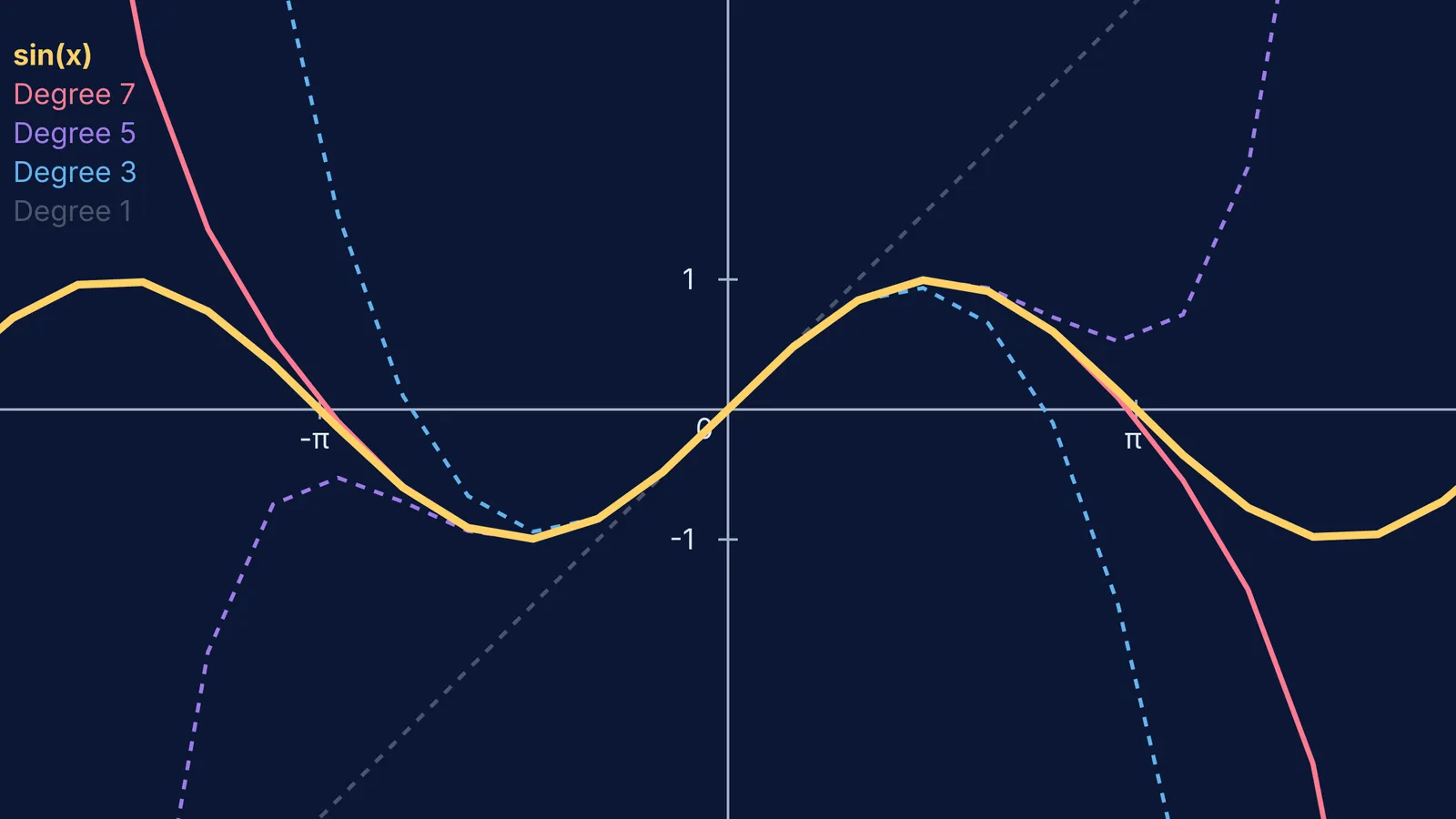
One term (degree 1): The polynomial is just y = x. This is a straight line that only matches the sine wave very close to the origin. It captures the initial slope of the wave but ignores its curvature.
Two terms (degree 3): Adding −x³/6 pulls the ends of the line down for positive x and up for negative x. This creates an S-shape that hugs the sine wave further out, capturing the first downward bend of the curve.
Three terms (degree 5): Adding x⁵/120 pulls the curve back up, pushing the accurate region just past the first peak of the sine wave.
Four terms (degree 7): By the time you add the −x⁷/5040 term, the polynomial wraps almost perfectly around the curve of sin x all the way past x = π and x = −π.
If you look closely at the simulation, each new term corrects the "overshoot" of the previous one. This alternating addition and subtraction creates a ripple effect that extends the accurate region further and further from the centre. This method is highly efficient for calculation. Charles Babbage's difference engine calculated sines, cosines, logarithms, and other transcendental functions by evaluating the first 7 terms of their Taylor series using the method of finite differences. Instead of performing complex multiplications, his mechanical engine found the answers through repeated addition, exploiting the properties of these polynomial approximations.
When does the approximation break down?
A finite Taylor polynomial will always eventually spiral away to infinity, because the highest power of x dominates the behaviour for large inputs. If you plot the 7th-degree polynomial for sine, it tracks the curve perfectly up to π, but by 2π it shoots sharply downwards to negative infinity, while the real sine wave simply returns to zero. To match the wave further out, you must add more and more terms. An infinite Taylor series matches the sine function everywhere, but in practice, calculators use a limited number of terms and rely on trigonometric identities to keep the input x small.
If you are struggling to picture how series expansions work, try plotting them yourself. Setting up the functions in a graphing tool and stepping through the terms builds an intuition that staring at equations cannot match. Watching the polynomial snake along the wave reveals the beautiful mechanics behind how we compute the world.