

On this page
Why can't a chimney filter just use a physical mesh?
When industrial boilers, cement kilns, and smelters burn fuel, exhaust carries microscopic soot and fly ash particles (PM10 and PM2.5). Why not simply place a fine HEPA fabric or mesh filter across the chimney stack to trap the smoke?
The obstacle is fluid mechanics. Chimneys discharge hundreds of cubic meters of exhaust per second. Forcing that volume through pores fine enough to trap 1-micrometre soot creates a crippling pressure drop. This back-pressure chokes combustion, strains ductwork, and demands megawatts of fan power. Moreover, sticky soot rapidly cakes over fabric pores, clogging the filter within hours.
In 1911, physical chemist Frederick Gardner Cottrell eliminated the physical barrier altogether. Publishing in the Journal of Industrial & Engineering Chemistry, Cottrell demonstrated that leaving the chimney channel open while applying a transverse electrical force sweeps particulates sideways out of the gas stream without impeding airflow.
How does an electrostatic precipitator charge and capture smoke particles?
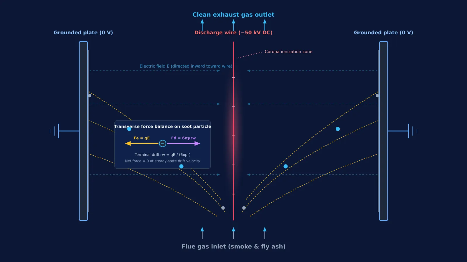
Technical specifications from the U.S. Environmental Protection Agency show that wire-plate electrostatic precipitators (ESPs) achieve 99% to 99.9% particulate removal efficiency while keeping pressure drop under 125 pascals. The system captures smoke in three steps:
Corona discharge: Discharge wires hang between vertical, grounded collector plates. A high-voltage direct-current supply charges the wires to −20 to −70 kilovolts (−20 to −70 kV). The wire's tight curvature produces an intense electric field exceeding air's breakdown limit of roughly 3 × 10⁶ V/m, generating a negative corona that emits electrons.
Particle charging: Electrons collide with gas molecules (such as O₂ and CO₂), creating negative ions that attach to upward-drifting smoke particles.
Collection: Charged particles experience a transverse force Fe = q · E, driving them toward grounded collector plates. As shown in our guide to electron deflection between charged plates, charged particles in transverse fields follow curved paths.
Periodic mechanical rapping knocks the collected ash layer into hoppers below, maintaining unobstructed gas flow.
How do plate voltage and particle charge determine drift velocity?
As analyzed in Aerosol and Air Quality Research, fluid friction opposes a charged smoke particle drifting sideways. By Stokes' law, the viscous drag force on a spherical particle of radius r moving at drift velocity w through gas of dynamic viscosity μ is Fd = 6π · μ · r · w.
Balancing electric force and viscous drag (q · E = 6π · μ · r · w) yields the terminal drift velocity:
w = (q · E) / (6π · μ · r)
This balance highlights why voltage is decisive:
For particles larger than 1 micrometre, field charging delivers a saturation charge q proportional to surface area (r²) and field strength E.
The electric field E scales with applied voltage V divided by plate spacing (E ≈ V / d).
Because acquired charge q and collecting field E both scale linearly with voltage, the electrostatic force Fe = q · E scales with the square of the voltage (V²). Doubling plate voltage quadruples the force driving soot toward the plates.
What happens to collection efficiency when you test higher voltages?
To relate drift velocity to total emissions, engineers use the Deutsch-Anderson equation, analyzed for fine particles in Aerosol and Air Quality Research:
η = 1 − exp(−A · w / Q)
Here, η is fractional collection efficiency, A is collecting plate area (in m²), w is drift velocity (in m/s), and Q is gas flow rate (in m³/s).
In a pilot chimney with gas flow Q = 10 m³/s and plate area A = 250 m²:
At low voltage (w₁ = 0.08 m/s): The exponent is −(250 × 0.08) / 10 = −2.0. Efficiency is η₁ = 1 − exp(−2.0) ≈ 86.47%. Over 13.5% of smoke escapes.
At medium voltage (w₂ = 0.18 m/s): The exponent becomes −4.5, yielding η₂ = 1 − exp(−4.5) ≈ 98.89%.
At peak voltage (w₃ = 0.28 m/s): The exponent reaches −7.0, delivering η₃ = 1 − exp(−7.0) ≈ 99.91%.
Raising drift velocity slashes escaping soot 150-fold. When working through electrostatics problems, students often confuse potential with field gradient; reviewing electrostatics mistakes in field and potential helps avoid sign errors. To practice similar step-by-step numericals, the Fermi Problem Library provides worked problems with a step-by-step solver that explains the reasoning rather than printing an answer.
How does predicting outcomes before running a simulation sharpen physics intuition?
Passive reading often masks conceptual gaps. The Predict-Observe-Explain (POE) framework, developed by Richard White and Richard Gunstone, prompts students to hypothesize before experimenting. A meta-analysis in the Proceedings of the National Academy of Sciences covering 225 studies found that active learning raised average STEM exam scores by roughly half a letter grade, while failure rates under traditional lecturing were 55% higher than under active learning.
You can apply this cycle to electrostatic precipitation:
Predict: If particle radius r is halved, will drift velocity increase or decrease? (Because field charge scales as r² while drag scales as r, smaller particles have lower drift velocity w ∝ r in the field-charging regime).
Test: Vary plate voltage and particle charge in a simulation to observe particle trajectories.
Explain: Contrast your predicted path with the simulated deflection and resolve any discrepancy.
Testing field forces dynamically clarifies principles that static sketches obscure, as explored in our guide to visualising electric and magnetic field lines. For ideas that are easier to see than to read, the Fermi Simulation Lab provides interactive simulations to explore physical models directly. To trace how these mechanics connect across topics, the Fermi Concept Library organizes every concept in physics and chemistry with its own lesson and place in the map.


