

On this page
A half-life graph in a textbook is a perfect smooth curve. Real decay is not smooth. Each nucleus decays at a moment nobody can predict, and the smooth curve only appears when you have a great many of them. A simulation lets you see both at once, and you can run one with coins on a table.
What does a radioactive decay simulation actually do?
It follows one rule. Split time into equal steps. In each step, every nucleus that has not yet decayed gets the same chance of decaying, and you decide each one separately, like a coin toss.
The rule comes from the physics. HyperPhysics describes radioactive decay as a statistical process that, for any given nucleus, is completely unpredictable. The number of nuclei that decay in a short time is proportional to the number still present, which gives N = N₀e^(−λt), where λ is the decay constant. It also gives the half-life as 0.693 times the mean lifetime 1/λ, so T½ = ln 2 / λ, about 0.693/λ.
If each step lasts one half-life, the chance per nucleus is exactly 1/2. If each step lasts a tenth of a half-life, the chance is 1 − (1/2)^0.1, about 0.067, which gives a smoother run.
How many nuclei remain after each half-life?
Start with N₀ = 1,000 nuclei. The expected number left after n half-lives is N₀ × (1/2)^n:
After 1 half-life: 500
After 2 half-lives: 250
After 3 half-lives: 125
After 4 half-lives: 62.5 on average, though any single run gives a whole number
After 5 half-lives: about 31
The chance that one particular nucleus survives three half-lives is (1/2)³ = 1/8. That is why about 1/8 of a large sample is left: the same probability, applied to many nuclei.
Why is radioactive decay random?
In 1910, Ernest Rutherford and Hans Geiger, with a mathematical note by Harry Bateman, counted the flashes made by alpha particles from a polonium source striking a zinc sulphide screen. They recorded 10,097 alpha particles over 2,608 intervals of 7.5 seconds, an average of 3.87 per interval.
They asked whether this scatter was what random emission would produce. The formula Bateman worked out for them, now known as the Poisson distribution, predicted 54 intervals with zero particles and 525 with three; the observed counts were 57 and 525. The authors concluded that the alpha particles are emitted at random. The scatter is not a fault in the equipment, and the smooth exponential is the average of many random events.
Why is the curve noisy for small samples?
Because the random wobble grows more slowly than the sample does. The same 1910 paper by Rutherford and Geiger cites E. von Schweidler's result that the typical error in a count is about the square root of the average count.
For decay over one half-life, the spread in the number remaining is √(N₀ × ½ × ½), the same as for heads in N₀ coin tosses:
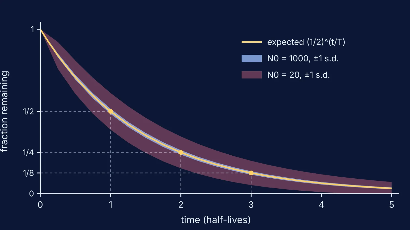
Start with 20 nuclei: expect 10 left, give or take about 2.2, so runs between 8 and 12 are ordinary. That spread is about 22% of the average.
Start with 1,000 nuclei: expect 500, give or take about 16, so typical runs fall between about 484 and 516. That spread is only about 3%.
The graph at the top shows this: the 20-nucleus band is wide, while the 1,000 band hugs the curve. If a 20-nucleus run has 4 nuclei left after three half-lives when the formula says 2.5, your simulation is not wrong.
How can you run the simulation yourself?
Put 100 coins in a tray. Each coin is one nucleus.
Write your predictions for after 1, 2, 3 and 4 throws: 50, 25, 12.5 and 6.25.
Shake the tray and tip the coins out. Remove every coin showing heads: those nuclei have decayed. Count the rest and write the number down.
Throw the survivors again, one throw per half-life, until none are left.
Plot your counts on top of the predicted curve. Then repeat with 20 coins and compare how far each run strays.
Try dice, with a six meaning decay. The chance per throw is 1/6, so using the half-life relation the half-life is ln 2 / ln(6/5), about 3.8 throws.
To code it instead, our guide to writing your own physics simulation in Python shows how to build a time-step loop; for decay, remove each nucleus when a random number falls below the decay chance. Predicting first is the same habit as in learning projectile motion with a simulation. For mean life and numericals, read the maths of radioactive decay and which exams test it.
The Fermi Simulation Lab has interactive simulations for the ideas that are easier to see than to read. If the jump from coin tosses to N = N₀e^(−λt) is where you get stuck, Fermi's AI tutor works out what you already know and builds a plan for the session.
Predict, toss, count: the gap between prediction and count is the lesson.


