

On this page
Projectile motion is one of the first places in JEE and NEET physics where two ideas have to work together: steady motion sideways and accelerated motion up and down. A simulation lets you fire hundreds of projectiles in minutes. But watching trajectories fly is not the same as learning from them. The trick is to predict before every launch. This post gives you a 30-minute activity with six predictions to test and a record sheet to keep.
Why predict before you press fire?
Crouch, Mazur and colleagues compared ways of showing physics demonstrations in class (American Journal of Physics, 2004). Students who only watched a demonstration understood the idea no better than students who did not see it at all. Students who predicted the outcome first showed significantly greater understanding. A simulation is a demonstration you control, so the same rule is worth applying: commit to a prediction, then look. For more on how simulations compare with diagrams, see simulations or static diagrams.
What you need
A projectile simulation. The free PhET Projectile Motion simulation from the University of Colorado lets you change initial height, angle, speed and mass, with and without air resistance (PhET Projectile Motion). Its stated learning goals include predicting how changing initial conditions affects a projectile's path and determining that the x and y motions are independent.
A notebook with three columns: My prediction and reason, What happened, Why.
The key results from your textbook, without air resistance and on level ground (OpenStax University Physics, section 4.3): range R = v₀² sin 2θ / g and time of flight T = 2v₀ sin θ / g, with horizontal and vertical motions independent.
Keep air resistance off for predictions 1 to 5.
Six predictions to test
1. Slow versus fast sideways launch
From a height of 10 m, launch horizontally (angle 0°) at 5 m/s, then at 15 m/s. Which lands first? Write your answer and reason. Then test, comparing the flight times shown by the simulation's tools or a stopwatch. Because vertical motion does not depend on horizontal speed, both should take about √(2h/g) ≈ 1.43 s; only the landing distance changes.
2. The angle for maximum range
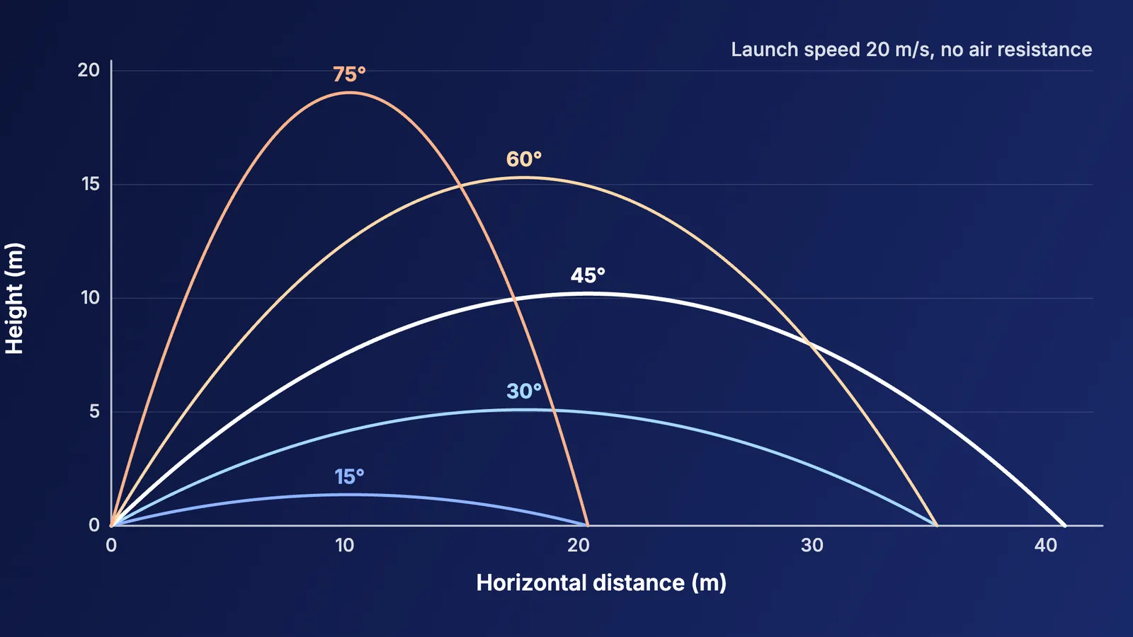
At a fixed speed of 20 m/s on level ground, which angle travels furthest? Predict, then try 30°, 40°, 45°, 50° and 60°. The formula says 45° gives the greatest range, about 40.8 m with g = 9.8 m/s². Small differences from the simulation may come from the value of g it uses and from rounding.
3. Two angles, one landing point
Predict the ranges at 30° and 60°: will the steeper shot land closer, further or at the same place? The formula says both reach about 35.3 m, because sin 60° = sin 120°. Now predict which stays in the air longer and goes higher. (60°: about 3.53 s and 15.3 m high; 30°: about 2.04 s and 5.1 m.) Same range, very different paths.
4. Double the speed
At 45°, what happens to the range if you double the launch speed? Since R depends on v₀², it should quadruple. Test 10 m/s against 20 m/s.
5. Heavier projectile
Without air resistance, does a heavier object go further? Look at the range formula: is mass in it? Predict, then switch between objects of different mass.
6. Turn air resistance on
Now you are beyond the textbook formula. Before testing, write predictions to three questions: Does mass now affect range? Is 45° still the best angle? Is the path still symmetrical? Then investigate, changing one setting at a time. There is no formula in your syllabus to lean on here, which makes it good practice in reasoning from forces: drag acts opposite to velocity, so think about what it does on the way up and on the way down.
After the simulation: turn it into exam skill
Explain each surprise in one sentence, in the Why column. For example: "Range depends on v₀², so doubling speed quadruples it."
Do three numerical problems on the same ideas without the simulation, checking with the formulas.
Sketch the graphs. Draw vertical velocity against time for prediction 3. It should be a straight line with slope −g for both shots, starting from a different initial value. Our guide on reading physics graphs shows how slopes and areas link to motion.
Revisit in a week. Redo predictions 3 and 4 from memory before reopening the simulation.
The Fermi Simulation Lab has interactive simulations for ideas that are easier to see than to read, and you can run the same predict-then-test routine there. Whatever tool you use, the habit is what does the work: predict, launch, explain.