

On this page
You walk away from a wall, stop, then walk back. Drawing it as a position-time graph, and then as a velocity-time graph, trips up a surprising number of good students. A walk-matching simulation is built to close that gap: you move a character, the graphs draw themselves as you go, and every guess you make gets checked straight away.
Why are motion graphs so hard to read?
In 1987, Lillian McDermott and colleagues described graphing errors from a multi-year study of several hundred university students in a laboratory-based preparatory physics course. Later testing found the same errors in other groups too (American Journal of Physics). They sorted the problems into two kinds: connecting graphs to physics concepts, and connecting graphs to the real world.
Robert Beichner's test of kinematics graphs collected data from 895 high school and college students (American Journal of Physics, 1994). The paper sums up a consistent set of difficulties that earlier research had found:
reading a graph as a picture of the path, as if a hill on the graph means the object went uphill
confusing slope with height, so "high on the graph" gets read as "fast"
trouble finding the slope of a line that does not pass through the origin
not knowing what the area under a curve means
Our guide to reading physics graphs covers slopes, areas and common misreadings.
How does a walk-matching simulation help?
Ronald Thornton and David Sokoloff described a motion detector that graphs a student's own movement in real time, and a kinematics curriculum built around it (American Journal of Physics, 1990). Using pre- and post-tests, they reported "strong evidence for significantly improved learning and retention" for students who used these materials, compared with those taught in lecture.
A simulation moves that sensor onto a screen. You drag or steer a character along a track, and the x-t and v-t graphs draw alongside. Or you work backwards: you are given a target graph and have to move the character so your line lands on it. The second is harder, because you must read the graph first. Our piece on when simulations beat static diagrams looks at what moving pictures add.
The Fermi Simulation Lab has interactive simulations for ideas that are easier to see than to read; the same predict-then-check habit works there.
What should you predict before you press play?
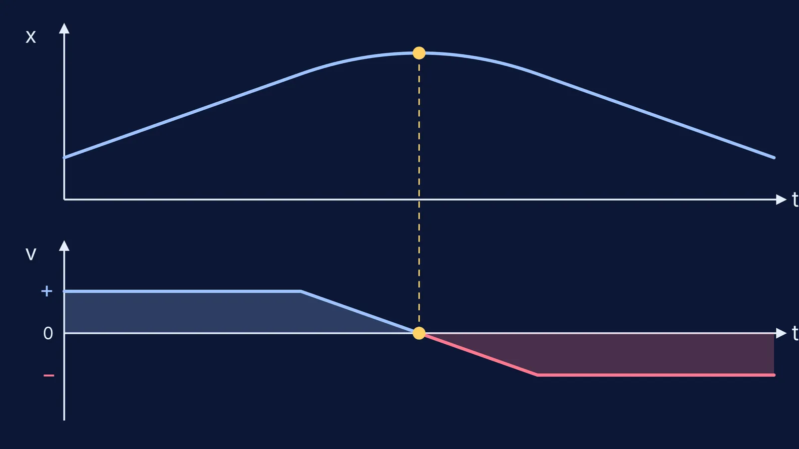
Take one walk, the one in the diagram above. The character starts 1 m from a wall. For 4 s it walks away at a steady 0.5 m/s. Then it slows down evenly, stops for an instant 3.5 m from the wall at t = 6 s, and comes back, reaching 0.5 m/s towards the wall at t = 8 s. It keeps that speed until t = 12 s, finishing at 1 m.
Before you run it, write down your answers:
What shape is the x-t graph from 0 to 4 s? A straight line sloping up, slope 0.5 m/s.
Where is the turning point on the x-t graph? At the top of the curve, t = 6 s, where the slope is zero.
What does the v-t graph show at that moment? It crosses the time axis. Velocity is zero.
Is acceleration zero at the turning point? No. The v-t line slopes down at the same rate from 4 s to 8 s, so acceleration is −0.25 m/s² the whole time, even at the instant the character is still.
What does the area under the v-t graph from 0 to 6 s give? 2.5 m, the distance from 1 m to 3.5 m.
Question 4 is a common slip. A ball thrown straight up also stops for an instant at the top, while gravity still acts.
What does a negative velocity look like?
Negative velocity means moving in the negative direction, here towards the wall. It does not mean slowing down. You can see it in three places:
On the x-t graph, the line slopes downwards. Position is getting smaller.
On the v-t graph, the line sits below the time axis.
In the simulation, the character moves back towards the start.
Try this: walk back towards the wall faster and faster. Velocity grows more negative while speed grows. If speed and velocity still blur together, our explainer on average speed versus average velocity helps.
How do you practise matching motion graphs?
Pick a target x-t graph. Sketch its v-t graph on paper first.
Say aloud what the character must do in each segment: "away, steady", "stop", "back, speeding up".
Run the walk and try to match the target. Note where your line drifts.
Compare your v-t sketch with the one the simulation drew. Circle every mismatch.
For each mismatch, name the mistake: slope or height, picture or graph, sign of velocity.
Repeat with a target v-t graph and predict the x-t graph.
If one mistake keeps coming back, Fermi's AI tutor can run the simulation with you and check your understanding as it goes.
Start with the walk above: predict, press play, and see which of your five answers held up.


