

On this page
If you have ever typed a log graph into a graphing tool and moved the base slider, you have seen the curve swing, flatten and flip. The useful part is guessing before you drag. Whether you are revising for school exams or JEE Main, here is what to predict, why it happens, and a short drill to run on yourself.
Where does a log graph cross the axis?
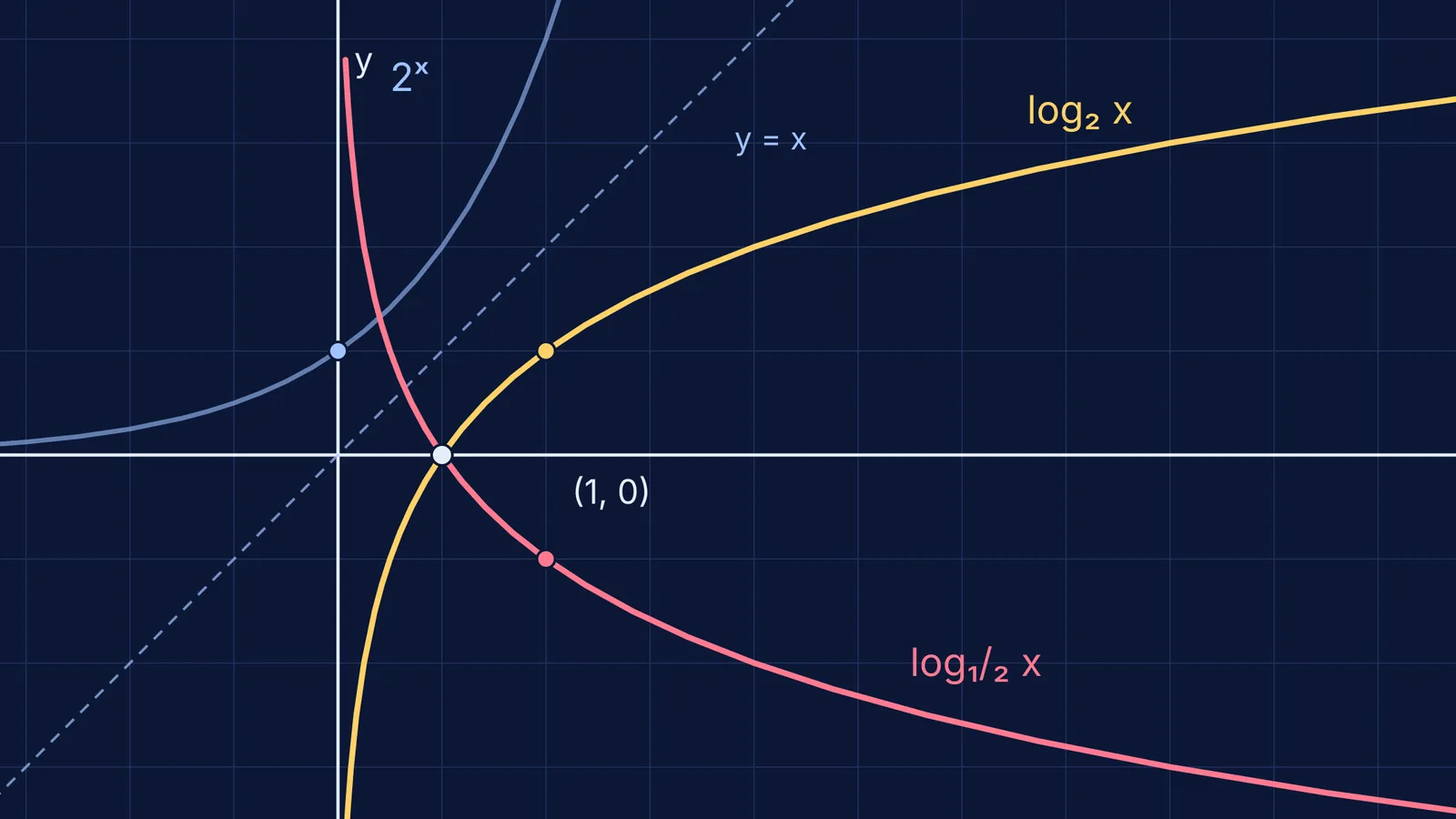
Every graph of y = log_b x crosses the x-axis at (1, 0), whatever the base, because b⁰ = 1 for any allowed base. OpenStax College Algebra 2e lists the key features: domain (0, ∞), range all real numbers, x-intercept (1, 0), vertical asymptote x = 0 and no y-intercept.
So when you slide the base, one point never moves. Watch (1, 0) stay pinned while the rest of the curve turns around it. The second useful point is (b, 1), since log_b b = 1. For base 3 the curve passes (3, 1) and (9, 2); for base 10 it only reaches 1 at x = 10.
How does the log graph mirror the exponential?
The graph of y = log_b x is the inverse of y = b^x, and the two graphs are reflections of each other across the line y = x, as the same OpenStax section on graphs of logarithmic functions shows. Swap the coordinates of any point on one and you get a point on the other: (0, 1) on y = 2^x becomes (1, 0) on y = log₂ x, and (3, 8) becomes (8, 3).
So the exponential's horizontal asymptote y = 0 becomes the log's vertical asymptote x = 0. For the general idea of reflecting a graph to find an inverse, our post on finding an inverse function and reflecting its graph works through more examples.
What happens to a log graph when the base is between 0 and 1?
The graph falls instead of rising: log_b x is increasing when b > 1 and decreasing when 0 < b < 1 (OpenStax). The change-of-base formula shows why. For positive b other than 1, log_b M = ln M / ln b (OpenStax, logarithmic properties). Since ln(1/2) = −ln 2, you get log₁/₂ x = −log₂ x. The base-½ graph is the base-2 graph flipped across the x-axis, still pinned at (1, 0).
The same formula explains two other things you will see on a slider:
Bases close to 1 give steep curves. ln b is close to 0, so you are dividing by a tiny number. Base 1.1 is far steeper than base 10.
Base 1 is missing. ln 1 = 0, so the formula breaks, and 1 raised to any power is 1, so y = 1^x has no inverse.
For bases between 0 and 1, the exponential and the log can even meet off the line y = x. With base 1/16, both curves pass through (1/2, 1/4) and (1/4, 1/2), because (1/16)^(1/2) = 1/4 and (1/16)^(1/4) = 1/2. Check it on paper before you trust the picture.
Why predict before you drag the slider?
Watching a slider move may teach little on its own. In a study of physics classroom demonstrations, Catherine Crouch, Eric Mazur and colleagues found that students who only watched understood the concepts no better than students who did not see the demonstration at all, while students who predicted the outcome first showed significantly greater understanding (Crouch et al., American Journal of Physics, 2004). A graph with a slider is a small demonstration, so the same habit applies.
The Fermi Simulation Lab has interactive simulations for ideas that are easier to see than to read. Use it the same way: say your prediction out loud before you change anything.
A five-minute prediction drill
Open any graphing tool with a slider for b (our guide to using graphing tools to learn functions, not skip them covers the setup). For each step, write your guess, then move the slider.
Set b = 2. Predict where the curve crosses the x-axis and its height at x = 8. (Answer: (1, 0) and 3.)
Change to b = 10. Predict whether the curve at x = 8 is higher or lower. (Lower: about 0.90.)
Change to b = 1.1. Predict steeper or flatter. (Much steeper: log₁.₁ 2 is about 7.3.)
Change to b = 0.5. Predict the shape. (The b = 2 curve flipped across the x-axis.)
Add y = b^x and y = x. Predict where the mirror shows, then try b = √2 and b = 1/16 from above.
When a prediction misses, write one line on why. If the gap is in the idea itself rather than the graph, the Fermi Concept Library gives every concept in mathematics its own lesson and its place in the map, so you can step back to exponents before returning to logs.
For the story of where all this began, read about John Napier and how logarithms turned multiplication into addition.


