

On this page
A heat conduction simulation lets you hold one end of a rod at 100 °C and the other at 0 °C, then watch the temperature settle along its length. It shows Fourier's law, the rule behind conduction questions in Class 11 and JEE Main, but only if you predict first. Here are the ideas, a worked example and six predictions to test.
What does the temperature profile look like in a rod at steady state?
Steady state means nothing is changing any more: every slice of the rod passes on exactly as much heat as it receives. The rate of conduction through a slab or rod is P = kA(Th − Tc)/d, where k is the material's thermal conductivity, A the cross-sectional area and d the thickness or length (OpenStax University Physics, section 1.6).
The same OpenStax section draws the consequence: with power and area constant, dT/dx is constant, so the temperature decreases linearly from the hot side to the cold side.
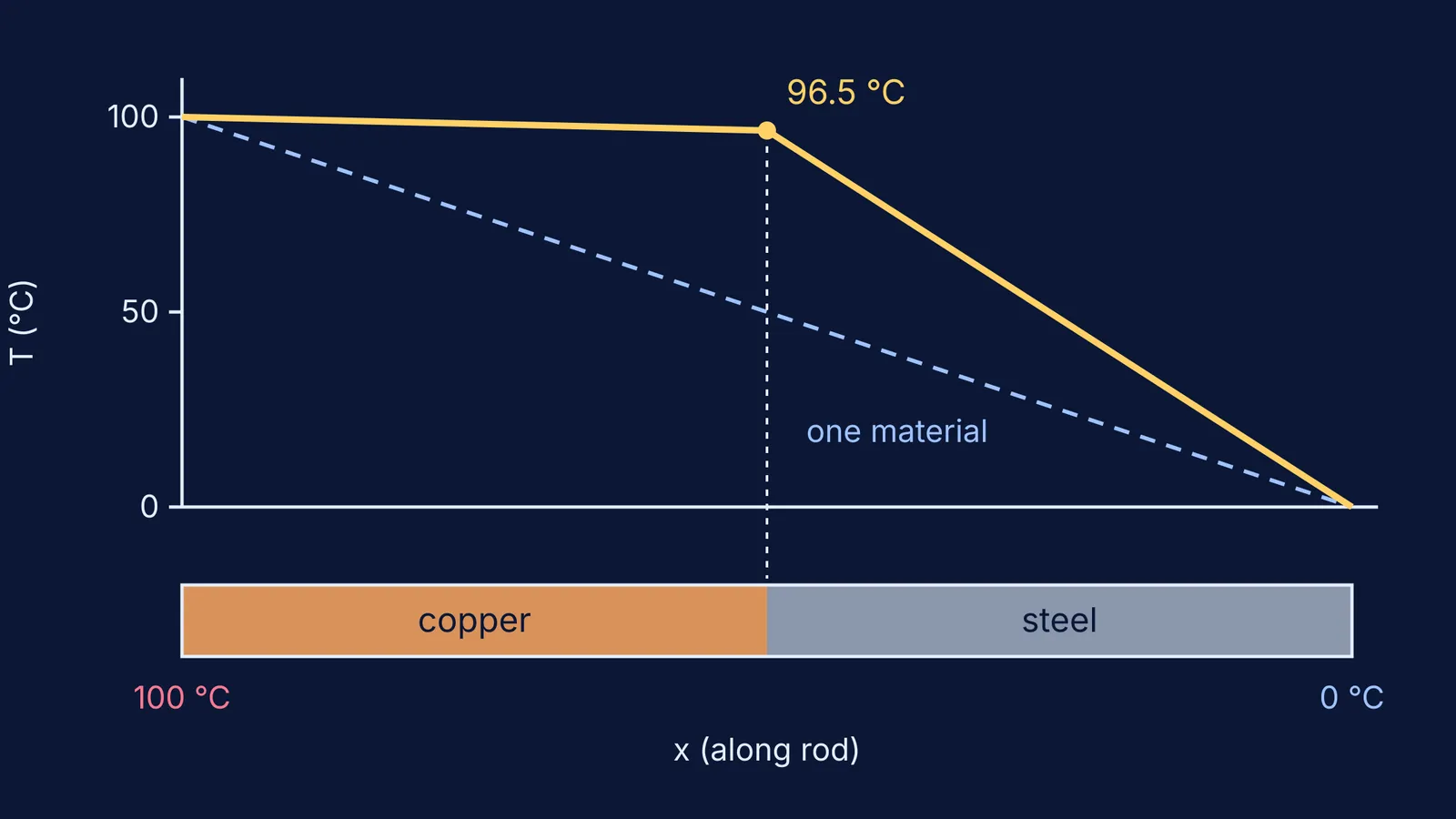
So for a rod of one material, the steady-state graph is the same straight line from 100 °C to 0 °C whether the rod is copper or steel. The material changes how much heat flows, not the shape of the line. Before steady state, a simulation shows a bent curve that straightens over time. The straight line assumes insulated sides; if the simulation lets the sides lose heat, the line sags into a curve.
How do length and area change the rate of heat flow?
The rate is proportional to area and to the temperature difference, and inversely proportional to length (OpenStax). OpenStax lists the thermal conductivity of copper as 390 W/m·°C, aluminium as 220 W/m·°C and stainless steel as 14 W/m·°C, with glass about 0.84 and air 0.023 (same source). Other tables differ slightly (HyperPhysics lists copper at 385 W/m·K), so use the values your question gives.
Worked example: a rod 0.5 m long with a cross-section of 1 cm² (10⁻⁴ m²), ends at 100 °C and 0 °C, using the OpenStax values above.
Copper: P = 390 × 10⁻⁴ × 100 / 0.5 = 7.8 W
Aluminium: P = 4.4 W
Stainless steel: P = 0.28 W
Double the length of the copper rod to 1 m and the rate drops to 3.9 W. Double the area instead and it rises to 15.6 W. The gradient along the rod also changes with length: 100 °C over 0.5 m is 200 °C per metre, but over 1 m it is only 100 °C per metre.
What is thermal resistance in heat conduction?
Rearrange the formula: Th − Tc = P × L/(kA). That has the shape of Ohm's law, V = IR, with temperature difference playing voltage and heat rate playing current. So thermal resistance is R = L/(kA), in kelvin per watt. OpenStax uses the closely related R factor, d/k, for insulation, and notes that the rate of heat transfer is inversely proportional to it (OpenStax).
In our example, the copper rod's R is 12.8 K/W and the stainless steel rod's is 357 K/W. Now join 0.25 m of copper to 0.25 m of steel, same area, ends at 100 °C and 0 °C. The resistances in series are 6.4 K/W and 178.6 K/W, which add to about 185 K/W. So P = 100/185 ≈ 0.54 W, and the copper loses only 0.54 × 6.4 ≈ 3.5 °C. The junction sits at about 96.5 °C: a nearly flat line through the copper, then a steep fall through the steel, as in the graph at the top.
For composite slabs, parallel paths and more practice, see our guide to thermal resistance and composite slab problems. For the person behind the law, read about Joseph Fourier and his theory of heat flow.
Six predictions to test in a heat conduction simulation
Write each prediction and a reason down before pressing play. Our summary of what PhET research says interactive simulations are good for explains why the predict-then-check habit matters.
Copper and steel rods, same size and end temperatures: will the steady-state temperature graphs differ? (No. Both are the same straight line.)
Which rod reaches steady state sooner? (Copper, typically.)
Double the length: what happens to the rate, and to the gradient? (Both halve.)
Double the area: what happens to the gradient? (Nothing. The rate doubles.)
Copper and steel joined end to end: where does the junction temperature sit, mid-range or near the hot end? (Near the hot end.)
Swap the order so steel is on the hot side: does the rate change? (No. Series resistances add in any order, but the junction moves near the cold end.)
If a result surprises you, explain it out loud using R = L/(kA) before moving on.
To see more ideas like this move, the Fermi Simulation Lab has interactive simulations for ideas that are easier to see than to read. And if a composite-rod problem still feels slippery, Fermi's AI tutor can draw the figure, run a simulation and check your understanding as you go.


