

On this page
When you first encounter graph transformations in Class 11 algebra or coordinate geometry for JEE, one pattern feels counterintuitive. If adding 2 to a function to form y = f(x) + 2 shifts the graph upward by 2 units, why does adding 2 inside the argument to form y = f(x + 2) shift the curve left rather than right? On the horizontal axis, positive values lie to the right, so moving left seems backwards.
The confusion comes from treating the algebraic addition as a command to the graph rather than an adjustment to the input. In a study published in *The Journal of Mathematical Behavior*, researchers Rina Zazkis, Peter Liljedahl, and Karen Gadowsky examined how 41 participants—comprising 16 practicing secondary mathematics teachers, 15 preservice teachers, and 10 high school students—explained horizontal translations of parabolas. They found that even experienced teachers relied on memorized rules to reverse the direction rather than explaining the underlying mathematics.
Why does adding to the input shift a graph to the left?
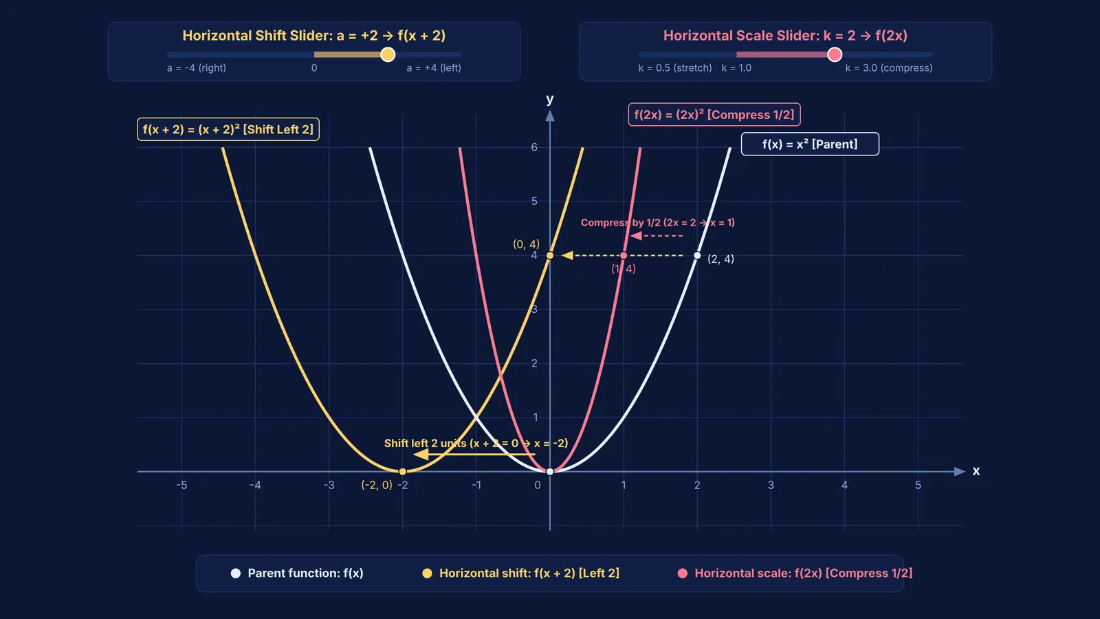
To understand why y = f(x + 2) moves left, track what happens to a single output. Take the vertex of the parent parabola y = f(x) = x², which occurs at x = 0 to give y = 0. In the transformed function y = f(x + 2), the function squares whatever value it receives. To produce that same output y = 0, the inner expression must equal zero: x + 2 = 0, so x = -2. The vertex now appears at x = -2 because adding 2 gives the input a head start.
Every point on the curve obeys this compensation. If you want the height the parent curve achieved at x = 4, your new input needs to be only x = 2, since f(2 + 2) = f(4). Because every output height occurs at an input 2 units smaller than before, the entire graph shifts 2 units to the left. Theodore Eisenberg and Tommy Dreyfus showed in Research in Collegiate Mathematics Education that students find horizontal transformations significantly harder to visualize than vertical ones because input modifications require solving an inverse problem before evaluating the function.
How do horizontal stretches and compressions work?
The same input compensation governs horizontal scaling. When you multiply the input by 2, as in y = f(2x), intuition might suggest that the graph doubles in width. Instead, the curve compresses horizontally by a factor of 1/2.
If f(x) reaches a peak at x = 6, the transformed curve f(2x) reaches that peak when 2x = 6, which gives x = 3. The curve reaches its features in half the horizontal distance. Conversely, y = f(x/2) stretches the graph horizontally by a factor of 2 because x must reach 12 before the inner argument evaluates to 6.
You can track these transformations systematically on the reference point (2, 4) of y = x²:
Horizontal shift y = (x + 2)²: solve x + 2 = 2 to get x = 0, moving (2, 4) left to (0, 4).
Vertical shift y = x² + 2: add 2 to the output height, moving (2, 4) up to (2, 6).
Horizontal compression y = (2x)²: solve 2x = 2 to get x = 1, moving (2, 4) inward to (1, 4).
Vertical stretch y = 2x²: multiply the output height by 2, moving (2, 4) up to (2, 8).
You can explore how these rules apply across functions in our guide to graph transformations for JEE.
How do interactive sliders build intuition through prediction?
Dynamic graphing sliders make these transformations visual, but passively sliding controls rarely builds lasting intuition. Real learning requires a predict-test cycle: commit to where a point will land on paper before touching the control.
A quasi-experimental study by Bulent Guven in the Australasian Journal of Educational Technology tracked 68 eighth-grade students across 36 experimental participants using dynamic geometry software and 32 control participants using static worksheets. Students using dynamic tools scored significantly higher on transformation geometry achievement tests by testing predictions against immediate visual feedback.
For strategies on combining algebraic reasoning with digital plots, explore using graphing tools to learn functions and calculus and our analysis of simulations or static diagrams.
How should you solve multi-step transformation problems?
To solve multi-step transformation problems without mixing up signs, use this three-step checklist:
Separate horizontal from vertical operations: check whether numbers modify x inside the function or modify the output outside.
Solve the input equation for the new x-coordinate: set the inner argument equal to key reference points (like roots or vertices) to find the exact horizontal shift or scale.
Apply vertical modifications directly: add or scale y without reversing signs.
When concepts are difficult to picture from equations alone, the Fermi Simulation Lab provides interactive simulations for ideas that are easier to see than to read. For composite problems combining horizontal shifts and scaling, the Fermi Problem Library offers worked problems with a step-by-step solver that explains the reasoning rather than just printing an answer.


