

On this page
Why does a fair coin game favour the richer player?
Imagine tossing an ordinary coin for 1 rupee per flip against an opponent holding 90 rupees, while you hold only 10 rupees. The total pot is 100 rupees. The coin is completely unbiased: heads adds 1 rupee, and tails subtracts 1 rupee. Intuition suggests that because every toss offers 50% odds, neither player has an advantage. Yet mathematical formulas compiled on Wolfram MathWorld prove that you will go broke in 90% of games, while your opponent wins the full 100 rupees in 9 out of 10 matches.
This asymmetry stems from absorbing boundaries. In a single flip, your expected gain is zero. But play continues until one person hits zero rupees. That zero is an absorbing barrier: once your bankroll empties, you cannot bet again. Starting with 10 rupees against 90 rupees leaves you only 10 steps from bankruptcy, while your rival is 90 steps away. Symmetric fluctuations touch the nearer boundary far earlier than the distant one.
This paradox was first explored in 1656 through letters between Blaise Pascal and Pierre de Fermat, analyzed by A. W. F. Edwards (1983) in the *International Statistical Review*. Christiaan Huygens published the first general solution in 1657, documented by Eddie Shoesmith (1986)90028-5) in *Historia Mathematica*.
How do you calculate the exact probability of ruin?
To determine ruin probabilities algebraically, express your wealth as a one-dimensional random walk with absorbing boundaries. Let P(k) be the probability of winning the entire pot of N rupees starting with k rupees. On the next coin toss, you either win 1 rupee with probability p or lose 1 rupee with probability q, where p + q = 1.
Conditioning on that flip gives the linear recurrence: P(k) = p × P(k + 1) + q × P(k − 1)
For a fair coin where p = q = 1/2: 2 P(k) = P(k + 1) + P(k − 1)
Rearranging terms shows that step differences are constant: P(k + 1) − P(k) = P(k) − P(k − 1)
Because differences are equal, P(k) forms an arithmetic progression. With boundary conditions P(0) = 0 and P(N) = 1, the closed-form solution is: P(k) = k / N
Your probability of ruin, R(k), is therefore: R(k) = 1 − P(k) = (N − k) / N
With k = 10 rupees and N = 100 rupees, your win chance is 10%, while your ruin chance is 90%. As derived in J. L. Coolidge's 1909 paper in *The Annals of Mathematics*, the expected duration in flips is E(k) = k(N − k). Starting with 10 rupees against 90 rupees means an average of 10 × 90 = 900 flips before someone goes broke. This recurrence also appears when solving probability in repeated-trial games in senior secondary maths.
What happens when you simulate 10,000 coin-toss games?
While algebraic proofs establish the 90% ruin figure, simulating thousands of games shows how individual trajectories behave. Running a Monte Carlo trial of 10,000 independent games with k = 10 and N = 100 demonstrates the law of large numbers:
Roughly 9,000 games terminate at 0 rupees.
About 1,000 games reach the 100-rupee target.
The average flip count per match converges to 900 steps, matching the theoretical expectation from J. L. Coolidge (1909).
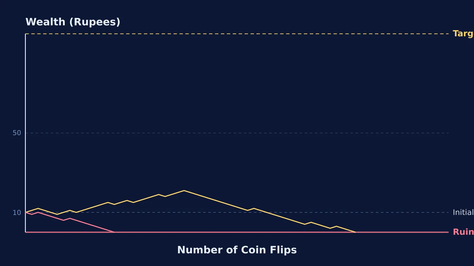
Plotting individual trajectories shows why intuition misleads. Losing runs rarely plunge straight to zero. Wealth wanders back and forth, often rising to 15 or 20 rupees before downswings drag it to zero.
When absorbing boundaries are hard to picture from static equations, interactive tools clarify the mechanics. The Fermi Simulation Lab provides interactive simulations for ideas that are easier to see than to read, allowing students to test parameter changes visually.
Why is casino ruin inevitable against infinite wealth?
When playing against an opponent with vastly superior reserves, such as a casino, the house's wealth is effectively infinite relative to your bankroll. Taking the limit as N approaches infinity shows: lim R(k) as N → ∞ = lim (N − k) / N = 1 − 0 = 1
Even in a game with fair 50-50 odds and zero house cut, playing indefinitely against infinite capital leads to bankruptcy with 100% certainty, as confirmed on Wolfram MathWorld. With no upper barrier to stop play, a symmetric random walk on integers eventually visits 0 with probability 1.
Real betting games are worse because they include a house edge, which severely slashes your win probability over long random walks. This steep drop explains why students often stumble on probability reasoning mistakes on competitive exams.
How can you test gambler's ruin step by step?
You can test these results in a simple Python experiment:
Set initial capital k = 10, target pot N = 100, and win probability p = 0.5.
Initialize counters for ruined games and total flips across 10,000 trials.
In each trial, simulate coin flips: add 1 rupee on heads and subtract 1 rupee on tails.
Stop the trial when wealth reaches 0 or 100 rupees, recording whether the run ended in ruin.
Divide total ruins by 10,000 to find the simulated ruin rate and average duration.
Running this test confirms the 90% ruin rate and 900-flip duration, matching the theory of absorbing Markov chains and the expectations derived by J. L. Coolidge (1909).
If you are working through probability numericals, the Fermi Problem Library has worked problems with a step-by-step solver that explains the reasoning rather than printing an answer.


