

On this page
It is tempting to drop the skater and just watch. That teaches less than it seems. In a 2004 study, Catherine Crouch, Eric Mazur and colleagues found that students who only watched a classroom demonstration understood the idea no better than students who never saw it, while students who predicted the outcome first showed significantly greater understanding (American Journal of Physics). So this guide gives you numbers to predict before you press play.
What does a skate park energy simulation show?
A widely used one is PhET's free Energy Skate Park. The listing for its simpler version, Energy Skate Park: Basics, invites you to "learn about conservation of energy" by watching kinetic energy, potential energy and friction as the skater moves, and its sample learning goals include "predict position or estimate speed from Energy Bar and Pie Charts" (PhET listing, CLIx platform at TISS). See also what PhET research says interactive simulations are good for.
Two ideas carry the whole simulation:
When height changes by h, gravitational potential energy changes by ΔPE = mgh (OpenStax College Physics 2e, 7.3).
When only conservative forces act, KE + PE at the start equals KE + PE at the end (OpenStax College Physics 2e, 7.6).
How fast is the skater at each height?
Set potential energy lost equal to kinetic energy gained: mgΔh = ½mv², so v = √(2gΔh), where Δh is the drop. When friction is negligible, final speed depends only on the starting speed and the height, not on the mass or the path taken (OpenStax 7.3). We use g = 9.80 m/s², the value OpenStax uses.
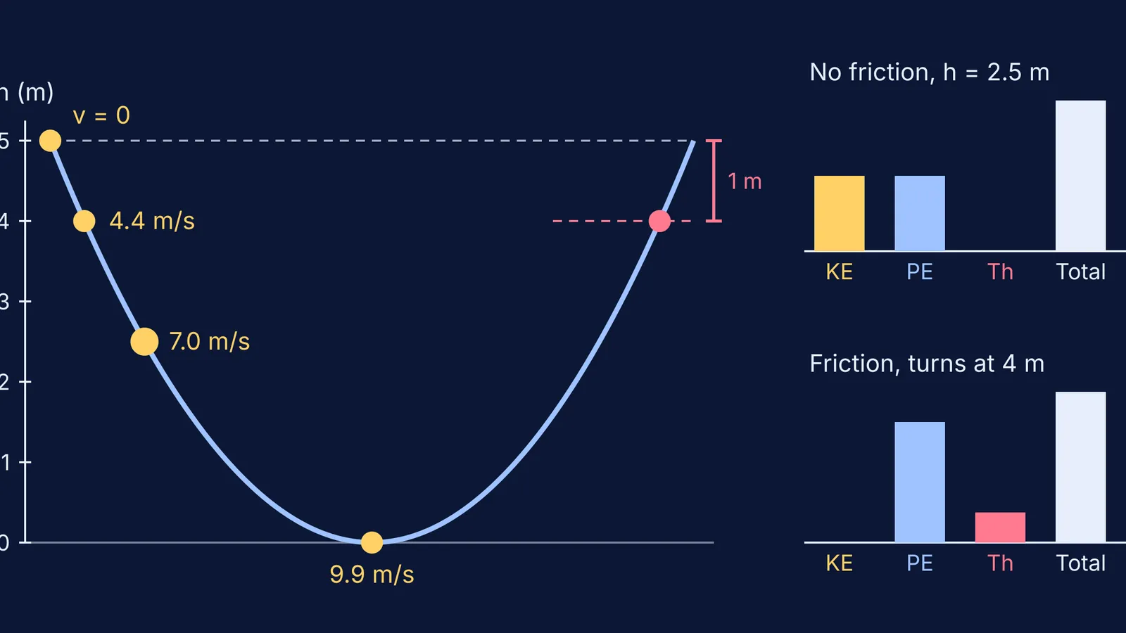
Worked example: a skater starts from rest at 5.0 m on a frictionless U-shaped track. Write these down before you look:
At 5.0 m: 0 m/s (a turning point)
At 4.0 m: √(2 × 9.80 × 1.0) = 4.4 m/s
At 2.5 m: √(2 × 9.80 × 2.5) = 7.0 m/s
At 0 m: √(2 × 9.80 × 5.0) = 9.9 m/s
The trap: halfway down, the skater has 7.0 of the final 9.9 m/s, about 71%, not half, because speed grows with the square root of the drop. Kinetic energy, not speed, is half at half height.
Then test two "nothing changes" predictions: double the mass, or reshape the track from the same start height. The bottom speed should stay 9.9 m/s.
How does the energy bar chart shift as the skater moves?
Take a 60 kg skater released from 5.0 m. Using ΔPE = mgh (OpenStax 7.3), the total is 60 × 9.80 × 5.0 = 2,940 J, with zero potential energy at the bottom of the track.
At the top: the PE bar is 2,940 J and the KE bar is empty.
At 2.5 m: the two bars are equal, 1,470 J each.
At the bottom: the KE bar is 2,940 J and the PE bar is empty.
Everywhere: the total bar does not move.
Moving the zero line for potential energy shifts the PE and total bars everywhere, but not the speeds. For the textbook side of KE and PE, see work and energy in Class 9.
Where does the lost energy go when friction is switched on?
Friction is a nonconservative force that dissipates mechanical energy as thermal energy (OpenStax College Physics 2e, 7.5), so the full equation becomes KEᵢ + PEᵢ + W_nc + OEᵢ = KE_f + PE_f + OE_f (OpenStax 7.6). On screen, a thermal bar grows while KE + PE shrink, and the total bar stays level. Predict first:
The skater no longer reaches 5.0 m on the far side.
The bottom speed is less than 9.9 m/s.
The thermal bar only grows, so the skater finally settles at the bottom.
Now measure. Suppose the skater turns at 4.0 m on the far side. There, KE is zero and PE is 60 × 9.80 × 4.0 = 2,352 J, so the thermal energy is 2,940 − 2,352 = 588 J, one fifth of the starting energy. That 4.0 m depends on the friction setting, so measure it rather than predict it.
How should you run the simulation, step by step?
Pick a start height and work out the total energy, mgh.
Predict speeds at three heights and sketch each bar chart.
Run with friction off and compare.
Change the mass, then the track shape, predicting "no change".
Switch friction on, measure the turning height and work out the thermal energy.
For every miss, write one sentence on why.
The same predict-then-check habit works for other motion topics, as in learning projectile motion with a simulation.
If you want more ideas that are easier to see than to read, the Fermi Simulation Lab has interactive simulations for the ideas that are easier to see than to read, and Fermi's AI tutor can run the simulation with you and check your understanding as it goes.
Start with the 5.0 m drop: write 4.4, 7.0 and 9.9 m/s on paper, the speeds from v = √(2gΔh) (OpenStax 7.3), then press play.


