

On this page
Open any spring or pendulum simulation, turn up the damping slider, and the wave on the graph starts to shrink. This post turns it into a short experiment: you make three predictions, run the simulation, and check them against the physics.
What does damping do to an oscillator's graph?
Damping is a force that opposes motion, usually modelled as proportional to velocity (F = −bv, where b is the damping constant). OpenStax University Physics, section 15.5 gives the lightly damped solution as x(t) = A₀e^(−bt/2m)cos(ωt + φ).
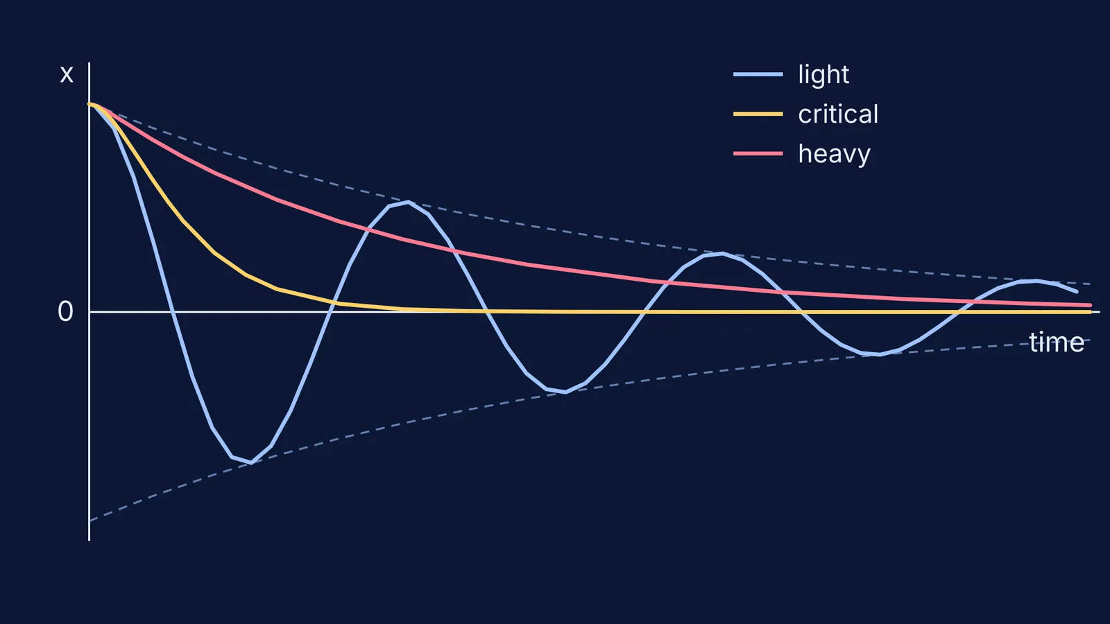
Read that equation as two parts multiplied together. The cosine is the oscillation you already know from SHM. The factor e^(−bt/2m) is an envelope that shrinks over time and squeezes the cosine between two curves. On the graph above, the dashed lines are that envelope, and the light blue curve keeps touching them.
How fast does amplitude decay in a damped oscillation?
The amplitude falls exponentially. That means it loses the same fraction every cycle, not the same number of centimetres. This is an easy prediction to get wrong.
A worked example using the OpenStax solution: take m = 0.5 kg, k = 50 N/m, b = 0.2 kg/s, and pull the block 10 cm from equilibrium.
Natural angular frequency: ω₀ = √(k/m) = 10 rad/s, so the undamped period is 2π/10 ≈ 0.628 s.
Decay rate: b/2m = 0.2 s⁻¹.
Amplitude ratio per cycle: e^(−0.2 × 0.628) ≈ 0.882. Each swing is about 88% of the one before.
Successive peaks: 10, 8.82, 7.78, 6.86, 6.05, 5.33 cm. The gaps shrink (1.18, 1.04, 0.92, 0.81, 0.72 cm) because each loss is a fixed share of a smaller amplitude.
Half the amplitude is gone after ln 2 / 0.2 ≈ 3.5 s, about five and a half cycles.
A quick check you can do on any graph: divide each peak by the one before it. If the ratio stays the same, the decay is exponential. If the differences stay the same instead, the damping is not proportional to velocity. Dry sliding friction, for example, gives a straight-line envelope.
Why does the period barely change with damping?
From the same OpenStax section, the damped angular frequency is ω = √(ω₀² − (b/2m)²). For small damping, OpenStax notes that the period and frequency are nearly the same as for SHM while the amplitude gradually decreases.
In our example, ω = √(100 − 0.04) ≈ 9.998 rad/s. The period grows from 0.6283 s to 0.6284 s, a change of about 0.02%, far too small for a stopwatch. The reason is that the damping term enters squared and is subtracted from ω₀². To change the period noticeably, b/2m has to become comparable to ω₀, and by then the motion hardly oscillates at all.
That finding comes from Crouch, Fagen, Callan and Mazur in the American Journal of Physics (2004). It is the reason this post asks you to write your predictions down before you run anything.
What do light, critical and heavy damping look like?
OpenStax defines critical damping as b = √(4mk). That condition is the same as b/2m = ω₀.
Light damping (b below √(4mk)): the curve crosses zero again and again, inside a shrinking exponential envelope.
Critical damping (b equal to √(4mk)): no crossing when released from rest. The system returns to equilibrium as fast as it can without overshooting. OpenStax uses car shock absorbers as the example.
Heavy damping (b above √(4mk)): still no crossing, but the return is slower than critical. The graph creeps towards zero.
In our example, critical damping needs b = √(4 × 0.5 × 50) = 10 kg/s. So b = 0.2 kg/s is just 2% of critical, which is why the motion keeps oscillating for so long.
The surprise for many students is that adding more damping past critical makes the system settle *more slowly*. On the hero graph, the pink (heavy) curve is still well above zero after the yellow (critical) curve has flattened out.
A five-step plan for any damping simulation
Use this with a pendulum, a spring-block or an LCR circuit.
Write down the undamped period before you touch the slider.
Predict the period with light damping. (It should be unchanged to the precision you can read.)
Predict the ratio of two successive peaks, then measure three ratios and check that they match.
Work out √(4mk) and predict the slider value where the curve stops crossing zero.
Double that value and predict whether the system settles faster or slower. Then run it.
If you get a prediction wrong, write one sentence explaining why before you move on.
The Fermi Simulation Lab has interactive simulations for ideas that are easier to see than to read, so you can test each prediction above on a moving graph. For the energy side of the same motion, read our guide to energy in SHM graphs. For the electrical version of damping, see LCR resonance and the quality factor. And for what research says about learning with simulations more broadly, see what PhET research says simulations are good for.


