

On this page
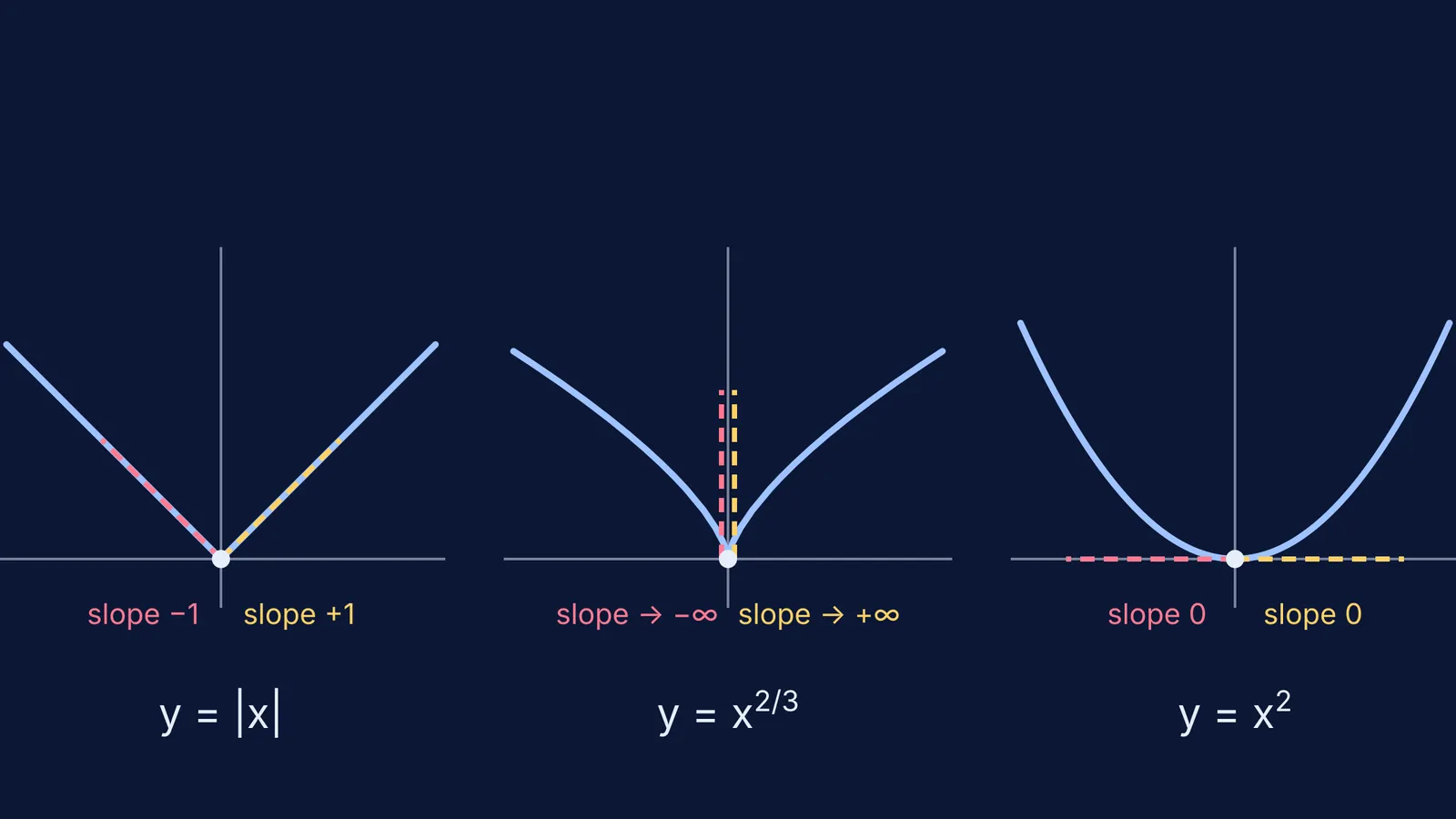
"Differentiable means continuous, but not the other way round" sticks better as a picture than as a sentence. Here you will zoom into a corner, a cusp and a smooth curve, and guess the left and right slopes before working them out.
What does continuous but not differentiable look like on a graph?
Continuous at a point means you can draw the graph through it without lifting your pen. Differentiable asks for more: the graph must have one tangent there, with a finite slope.
The NCERT Class 12 textbook defines a function as differentiable at c if the left-hand and right-hand limits of [f(c + h) − f(c)]/h, as h → 0, are both finite and equal (NCERT Mathematics Part I, Chapter 5). The same chapter proves that every differentiable function is continuous, and notes that the converse is not true, using f(x) = |x| as the example.
OpenStax's calculus textbook lists the ways a function can fail to be differentiable at a point: a sharp corner, a vertical tangent, rapid oscillation, or a discontinuity (OpenStax Calculus Volume 1, section 3.2). Only the last breaks continuity: corners, vertical tangents and oscillation can all happen on a graph you draw without lifting your pen.
Why is |x| not differentiable at x = 0?
Predict first. Look at the V shape. To the left of 0 the graph is the line y = −x, so the slope there should be −1. To the right it is y = x, so the slope should be +1.
Now compute. For h < 0, [f(0 + h) − f(0)]/h = |h|/h = −h/h = −1. For h > 0 it is h/h = +1. These are exactly the left-hand and right-hand limits worked out in the NCERT chapter, and because −1 ≠ +1 the derivative at 0 does not exist.
The visual test: zoom into |x| at the origin and you see the same V at every magnification. The corner never goes away, so no single tangent fits.
How is a cusp different from a corner?
Take y = x^(2/3). It is continuous at 0, but the graph comes to a sharp point. An open precalculus text describes this cusp: near x = 0 the tangent lines get steeper and steeper, with a negative slope on one side and a positive slope on the other (Lumen Learning, Derivatives).
Predict: on the left the curve dives steeply down into the origin, so the slope should be large and negative. On the right it climbs steeply, so large and positive.
Compute: [f(h) − f(0)]/h = |h|^(2/3)/h. Put in h = 0.001 and you get 10. Put in h = −0.001 and you get −10. With h = ±0.000001 you get ±100. The one-sided slopes do not settle on any finite number: they head to −∞ and +∞.
Zooming shows the difference from |x|. If you magnify the graph by a factor k in both directions, y = x^(2/3) turns into y = k^(1/3) x^(2/3), which is steeper. A cusp gets sharper the closer you look.
Why does a smooth curve pass the zoom test?
Now y = x² at 0. Predict: the bottom of the bowl is flat, so both slopes should be 0. Compute: [h² − 0]/h = h, which goes to 0 from both sides. The left and right slopes agree, so the derivative exists and equals 0. Zoom in and the bowl straightens into the x-axis.
So: a corner gives two different finite slopes, a cusp gives slopes running to opposite infinities, and a smooth point gives one slope from both sides.
How do you check any point for a corner?
Use this four-step routine on a JEE or board question.
Find the suspicious points: where the expression inside a modulus is zero, where a piecewise rule switches, or where a fractional power meets 0.
Check continuity there first. If the graph jumps, it is not differentiable and you are done.
Sketch the graph near the point and predict the sign and rough size of each one-sided slope.
Compute the left-hand and right-hand limits of the difference quotient and compare them with your prediction.
Worked example: f(x) = |x² − 4| at x = 2. Just left of 2, x² − 4 is negative, so f(x) = 4 − x² and the slope approaches −2(2) = −4. Just right of 2, f(x) = x² − 4 and the slope approaches 2(2) = +4. The graph is continuous, but −4 ≠ +4, so there is a corner. At x = 0, by contrast, f(x) = 4 − x² on both sides and the slope is 0: smooth.
For step 2, see removable and jump discontinuities; for more practice, differentiability for JEE; and for predicting before you plot, using graphing tools to learn functions and calculus.
TheFermi Simulation Lab has interactive simulations for the ideas that are easier to see than to read. If the definition of a limit itself is the shaky part, the Fermi Concept Library has a lesson for each concept in mathematics.


