

On this page
In October 1897 J. J. Thomson published a paper called "Cathode Rays" in the Philosophical Magazine (Thomson, 1897). Its method still works in a simulation: compare an electric bend with a magnetic one to get the beam's speed, then the charge-to-mass ratio.
How did Thomson measure e/m of the electron?
Thomson sent cathode rays between two parallel aluminium plates "about 5 cm. long by 2 broad and at a distance of 1.5 cm. apart", and read the glowing spot's shift on a scale (full text of the paper). Two coils outside the tube added a magnetic field over the same stretch. In modern symbols (he wrote F and H):
With only the electric field E, acting over a length l, the beam turns through an angle θ = (e/m)·E·l/v².
With only the magnetic field B, it turns through an angle φ = (e/m)·B·l/v.
Thomson adjusted the coil current until the magnetic bend equalled the electric bend, φ = θ. Then v = E/B, and m/e = B²l/(Eθ).
Turn the last formula upside down and you get the one you will use: e/m = Eθ/(B²l).
His table gave m/e of 1.1 to 1.5 × 10⁻⁷ in CGS units for air, hydrogen and carbonic acid. He concluded the value "is independent of the nature of the gas" and very small next to 10⁻⁴ for the hydrogen ion in electrolysis, a thousand times smaller (Thomson, 1897).
The electron's charge-to-mass ratio is −1.758 820 008 38 × 10¹¹ C/kg (CODATA 2022, NIST). In SI, Thomson's numbers come to roughly 0.7 to 0.9 × 10¹¹ C/kg, about half that value or a little less. He flagged one source of error himself: he ignored the reversed magnetic field outside the plates, which made his m/e values too large. The full story is in how Thomson arrived at the electron.
How do you run Thomson's experiment in a simulation?
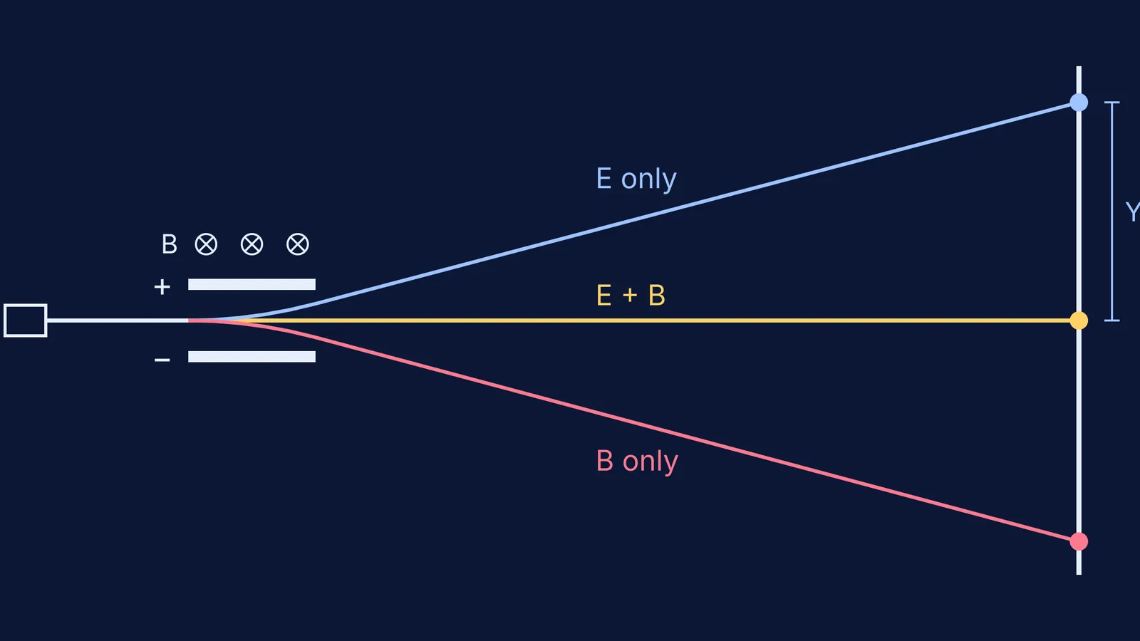
Most simulations tune both fields until the beam runs straight, which gives the same v = E/B as Thomson's equal bends. Write each prediction down before you click.
Fields off. Predict: the spot lands dead centre.
Top plate positive. The negative electron moves toward the positive plate. Record the spot's shift Y.
Predict the path: a parabola between the plates, then a straight line, as in electron deflection between charged plates.
E off, B on, pointing into the page (away from you), with the beam moving left to right. Use F = qv × B with negative q: the beam curves down along a circular arc.
Both on. Raise B until the spot is back at centre. Now eE = evB, so v = E/B, the idea behind a velocity selector with crossed E and B fields. Record B.
Work out e/m, change the voltage and repeat.
What e/m do you get? A worked example
Say your simulation copies the size of Thomson's plates (Thomson, 1897): length l = 5.0 cm, gap d = 1.5 cm. Put 200 V across them and a screen L = 30 cm past the end of the plates.
Field: E = V/d = 200/0.015 = 1.33 × 10⁴ V/m.
With only the electric field on, the spot moves up by Y = 53.6 mm.
Balance: the spot returns to the centre at B = 0.50 mT. So v = E/B = (1.33 × 10⁴)/(5.0 × 10⁻⁴) = 2.67 × 10⁷ m/s.
Angle: trace the straight part of the path back and it seems to start from the middle of the plates. So θ ≈ Y/(l/2 + L) = 53.6/(25 + 300) = 0.165 rad.
Ratio: e/m = Eθ/(B²l) = (1.33 × 10⁴ × 0.165)/((5.0 × 10⁻⁴)² × 0.050) ≈ 1.76 × 10¹¹ C/kg.
We worked out these readings from the NIST value, so this tests your method rather than making a new measurement. The speed is realistic: Thomson's table lists 2.2 to 3.6 × 10⁹ cm/s, which is 2.2 to 3.6 × 10⁷ m/s (Thomson, 1897).
What mistakes do students make with e/m problems?
Bending the wrong way. The right-hand rule is for positive charges; flip it for electrons.
Calling the magnetic path a parabola. It is a circular arc, because the force stays at right angles to the velocity.
Reading mT as T. B is squared, so a slip of 1000 in B becomes a slip of a million in e/m.
Measuring θ from the end of the plates. In the worked example above, Y/L gives 0.179 rad and an e/m about 8% too high. Use Y/(l/2 + L).
If crossed fields are still hard to picture, the Fermi Simulation Lab has interactive simulations for ideas that are easier to see than to read. If you get stuck on step 4, Fermi's AI tutor can draw the figure and run the simulation with you, checking your understanding as it goes. Predict first, then let the screen tell you.


