On this page
A coin-toss simulation is one of the quickest ways to watch probability turn into a shape. You toss some coins, count the heads and repeat hundreds of times. The tallies build a histogram whose shape you can predict before you press run.
What does a binomial distribution simulation actually do?
Each run tosses n coins. Each coin lands heads with probability p, and the coins do not affect each other. The number of heads in one run is a binomial random variable. The NIST/SEMATECH e-Handbook of Statistical Methods describes the binomial distribution as the one to use when a trial has exactly two mutually exclusive outcomes, labelled success and failure.
The same handbook gives the two numbers that describe the histogram:
The mean of a binomial distribution is np (NIST/SEMATECH).
The standard deviation of a binomial distribution is √(np(1−p)) (NIST/SEMATECH).
The simulation never uses these formulas; it just tosses coins, so a prediction that matches the bars shows you understand them.
If mean and variance of a random variable still feel shaky, our walkthrough of probability distributions for JEE, with mean and variance worked out covers the groundwork.
What shape should the coin-toss histogram have?
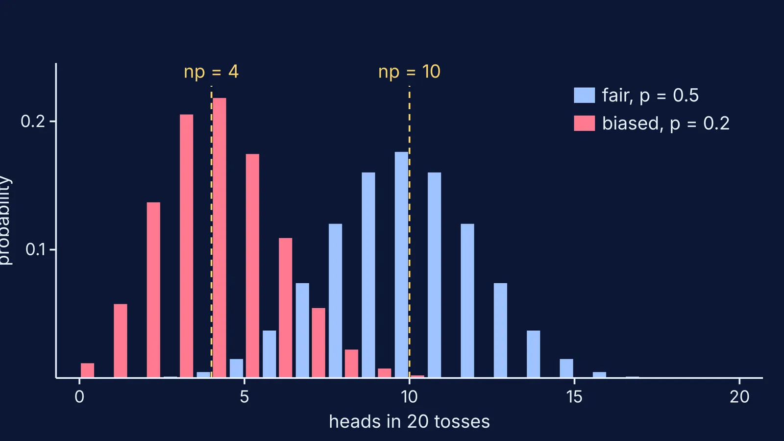
Take n = 20 fair coins (p = 0.5) and 1,000 runs. Work it out on paper first with the NIST/SEMATECH binomial formulas.
Centre: np = 20 × 0.5 = 10 heads.
Spread: √(20 × 0.5 × 0.5) = √5, about 2.2 heads.
Shape: symmetric. The chance of k heads equals the chance of k tails, so the left and right halves mirror each other.
Tallest bar: P(10 heads) = C(20,10)/2²⁰ = 184,756/1,048,576, about 0.176. Over 1,000 runs, expect roughly 176 runs to land on exactly 10.
Now run it. Your bar at 10 will not be exactly 176. Whether a run lands on 10 is itself a yes-or-no trial, so the bar's height follows a binomial with n = 1,000 and p = 0.176. Its standard deviation is √(1000 × 0.176 × 0.824), about 12. So anything from about 152 to 200 is normal noise, not a broken simulation.
How does a biased coin skew the histogram?
Now make the coin land heads only 20% of the time: p = 0.2, still with 20 coins. The same NIST/SEMATECH formulas give:
Centre: np = 20 × 0.2 = 4 heads.
Spread: √(20 × 0.2 × 0.8) = √3.2, about 1.8 heads, narrower than the fair coin's.
Tallest bar: k = 4, with probability about 0.218.
Shape: lopsided. The count cannot go below 0, which is only about two standard deviations from the centre, but it can stretch up to 8, 9 or 10.
The handbook gives the binomial skewness as (1−2p)/√(np(1−p)) (NIST/SEMATECH). For p = 0.5 the top is zero, so there is no skew. For p = 0.2 it comes to 0.6/1.79, about 0.34: positive, meaning the long tail is on the right. Flip it to p = 0.8 and you get the mirror image, with the tail on the left.
When does the histogram look like a bell curve?
More coins per run make the shape smoother and more symmetric, even for a biased coin. Online Statistics Education gives a rule of thumb: the normal approximation to the binomial is good if both np and n(1−p) are greater than 10.
The fair coin has np = 10, right at the edge of that rule, and it already looks close to a bell. The biased coin has np = 4, so the skew is easy to see. Raise the biased coin to n = 100 and np = 20, n(1−p) = 80: the histogram centres on 20, spreads by √16 = 4, and looks much more like a bell.
Our piece on Jacob Bernoulli and the law of large numbers, with coin-toss maths explains why averages settle down as runs pile up.
A five-minute prediction routine
Use this whenever you change a setting in a simulation:
Write n and p.
Work out np. This is where the peak should sit.
Work out √(np(1−p)). Most bars should fall within about two of these on each side of the centre.
Decide the lean: no tail if p = 0.5, a right tail if p is below 0.5, a left tail if p is above 0.5.
Check np and n(1−p) against the rule of thumb of 10 to guess how bell-like the shape will be.
Run 1,000 trials and compare. If a prediction fails, find which step went wrong before changing anything else.
For when watching a process build up beats a finished figure, see our look at simulations versus static diagrams.
The Fermi Simulation Lab has interactive simulations for the ideas that are easier to see than to read. If a binomial exam question still trips you up, the Fermi Problem Library has worked problems with a step-by-step solver that explains the reasoning rather than printing an answer.