On this page
What happens to air pressure as you climb from Mumbai to Everest?
Imagine standing at sea level along Marine Drive in Mumbai. The barometric pressure resting on your shoulders is roughly 101.3 kPa (1,013 hPa), standard sea-level pressure defined by the U.S. Standard Atmosphere (1976). Now imagine ascending to Mount Everest’s summit at 8,849 metres. Before checking data or setting up an integral, what would you guess the air pressure is at the peak?
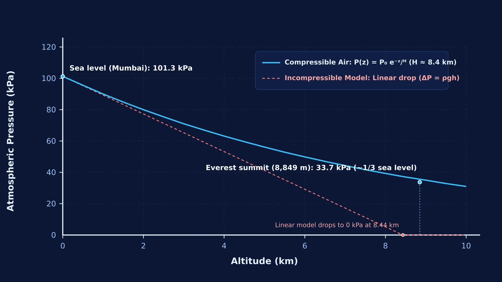
Most students guess that pressure drops by half, or that it dwindles to near zero because the air feels impossibly thin. During the 1981 American Medical Research Expedition to Everest led by John B. West, expedition physician Christopher Pizzo took direct barometric readings on the summit and measured 253.0 Torr, or approximately 33.7 kPa (West et al., 1983). Modern automated weather stations analyzed by Matthews et al. (2020) recorded a long-term mean summit pressure of 331 hPa (33.1 kPa). On the highest point of Earth, the air pressure is almost exactly one-third of what you feel in Mumbai.
That altitude reduces air pressure has been known since the seventeenth century, when Blaise Pascal: pressure, a mountain barometer and probability documented the first mountain barometer experiment on the Puy de Dôme in 1648. Yet the shape of that decline regularly catches physics students off guard.
Why does intuition fail when predicting altitude pressure?
Our daily intuition about fluid pressure comes from water. When you dive underwater in a swimming pool, hydrostatic pressure increases linearly with depth according to ΔP = ρ × g × h. Water is essentially incompressible: its density ρ remains constant whether you are near the surface or deep below.
If atmospheric air behaved like water with a uniform sea-level density of 1.225 kg/m³ (U.S. Standard Atmosphere (1976)), the entire atmosphere would run out where P = 0. Dividing 101,325 Pa by (1.225 kg/m³ × 9.807 m/s²) gives a total atmospheric height of only 8,435 metres (8.44 km). Under that linear assumption, Mount Everest at 8,849 metres would protrude past the top of the atmosphere into a vacuum.
In reality, air is a compressible gas. The ideal gas law shows that air density depends directly on pressure:
ρ = (P × M) / (R × T)
Here M is the mean molar mass of dry air (roughly 28.96 g/mol, as derived in our guide on the average molar mass of a gas mixture), R is 8.314 J/(mol·K), and T is absolute temperature.
Because lower layers must support the weight of all the air stacked above them, they are compressed tightly. As you climb upward, less air remains overhead, so the air expands and density drops. Substituting density into the hydrostatic differential equation dP/dz = −ρ × g yields:
dP / P = −(M × g / (R × T)) dz
Integrating this relation reveals that atmospheric pressure falls exponentially: P(z) = P₀ × exp(−z / H), where the scale height H = (R × T) / (M × g) is approximately 8.4 kilometres.
How does an interactive simulation change how you learn the curve?
Looking at an exponential formula on a blackboard rarely corrects stubborn linear intuition. Research by Sokoloff and Thornton (1997) on interactive learning found that asking students to commit to a written prediction before observing a physical demonstration lifted conceptual understanding from typical lecture gains of 10–20% to over 80%. When your brain explicitly commits to a wrong number, the surprising discrepancy forces you to revise your mental model.
Digital simulations make that cycle immediate. In a landmark paper on interactive simulations, Wieman, Adams, and Perkins (2008) highlighted how interactive environments allow students to manipulate variables and connect invisible microscopic particle density with macroscopic gauges, a dynamic explored further in what PhET research says interactive physics simulations are good for.
For concepts that are easier to see than to read, the Fermi Simulation Lab provides interactive simulations where you can adjust altitude, watching gas density thin out while tracking pressure changes in real time. If you run into wrong-method mistakes on atmospheric physics problems, the Fermi Problem Library offers worked problems with a step-by-step solver that explains the reasoning rather than printing an answer. When you encounter broader concept gaps, the Fermi Concept Library covers every concept in physics, chemistry, biology, mathematics and computing, each with its own lesson and its place in the map.
What is the step-by-step framework to test your atmospheric model?
To get the most out of an altitude simulation, use this three-step Predict-Observe-Explain routine based on the U.S. Standard Atmosphere (1976) model before touching the controls:
Predict the values in your notebook: Write down your estimates for three checkpoints: Bengaluru (roughly 900 m elevation), Mount Everest Base Camp (5,364 m), and Everest Summit (8,849 m). Calculate what an incompressible linear model predicts at each point: P_linear = 101.3 − (12.0 × h_km) kPa.
Observe the simulated ascent: Climb to 1,000 m. Notice that pressure drops by roughly 11.4 kPa in the first kilometre. Now climb from 7,000 m to 8,000 m. Even though the climb is the same 1,000 vertical metres, pressure drops by only about 5.5 kPa. The curve is steep near sea level where air is dense, and flattens out higher up where molecules are sparse.
Explain the discrepancies with the barometric equation: Calculate the isothermal estimate for Everest: P = 101.3 × exp(−8.849 / 8.43) ≈ 35.4 kPa. When factoring in the standard tropospheric temperature lapse rate of −6.5 K/km from the U.S. Standard Atmosphere (1976), the model yields approximately 31.4 kPa. The actual summit pressure measured by expedition physician Christopher Pizzo was 253.0 Torr (33.7 kPa, West et al., 1983), while weather station records report a long-term mean of 331 hPa (Matthews et al., 2020)—higher than global models because subtropical air columns are warmer and thicker.
Testing your prediction against the simulation turns an abstract formula into an unforgettable physical landscape.