

On this page
When Norwegian explorer Fridtjof Nansen froze his wooden schooner *Fram* into Arctic pack ice in 1893, he expected drifting ice to follow the prevailing winds. Instead, his daily navigational records, published in The Norwegian North Polar Expedition Scientific Results, revealed an unexpected puzzle: pack ice consistently drifted 20° to 40° to the right of the wind direction.
Nansen suspected Earth's rotation was deflecting the ice, but could not solve the fluid dynamics himself. In 1901, he described the problem to Norwegian meteorologist Vilhelm Bjerknes and atmospheric physics. Bjerknes passed the challenge to his 27-year-old doctoral student, Swedish physicist Vagn Walfrid Ekman. In 1905, Ekman published the complete mathematical solution, demonstrating how winds drive a spiraling staircase of currents beneath the sea.
Why did Arctic ice drift away from the wind?
In everyday mechanics, pushing an object moves it directly in line with the force. In the ocean, however, water moves on a rotating sphere. Any moving parcel of fluid experiences an apparent acceleration perpendicular to its path—the sideways Coriolis deflection.
When wind blows across open water, it exerts horizontal wind stress on the surface layer. As surface water moves forward, Coriolis acceleration deflects it to the right in the Northern Hemisphere (and to the left in the Southern Hemisphere). Nansen observed this directly because Arctic ice floes rested on top of this turning boundary layer. Water's viscosity then drags each underlying layer forward while transferring momentum downward.
How does the Ekman spiral rotate with depth?
To model the water column, Ekman set up a steady-state balance, analyzed by Earth Sciences History, between internal shear friction (vertical eddy viscosity K_z) and the Coriolis force (parameter f = 2 Ω sin ϕ, with Earth's angular speed Ω and latitude ϕ).
The resulting equations describe the classic Ekman spiral:
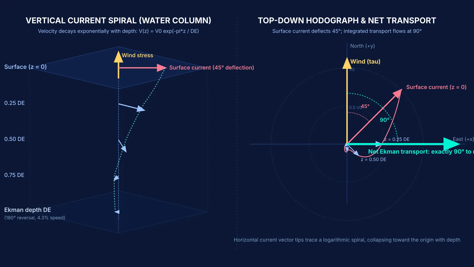
At the surface, current flows at 45° to the right of the wind in the Northern Hemisphere.
Each successive deeper layer moves more slowly and turns further to the right.
Current speed decays exponentially with depth as exp(−π z / D_E), where D_E is the depth of frictional influence.
At depth D_E, current direction reverses 180° relative to the surface, with speed dropping to e⁻π, or roughly 4.3% of the surface value.
Integrating velocity over depth reveals that total net water movement—Ekman transport—flows at exactly 90° to the right of the wind in the Northern Hemisphere (and 90° to the left in the Southern Hemisphere).
Visualizing how velocity vectors twist and decay beneath the surface is difficult from static equations alone. The Fermi Simulation Lab has interactive simulations for ideas easier to see than read, letting you observe how changing latitude and eddy viscosity alters rotating fluid layers.
How do you calculate the Ekman layer depth?
You can calculate the Ekman layer depth D_E using the classical relation from Ekman's 1905 derivation:
D_E = π × √(2 K_z / |f|)
For open-ocean conditions at latitude ϕ = 30° N:
Identify the Coriolis parameter: Using Ω = 7.292 × 10⁻⁵ rad/s, f = 2 × (7.292 × 10⁻⁵ rad/s) × sin(30°) = 7.292 × 10⁻⁵ s⁻¹.
Choose eddy viscosity: Turbulent mixing yields roughly K_z = 0.02 m²/s (200 cm²/s).
Compute 2 K_z / f: (2 × 0.02 m²/s) / (7.292 × 10⁻⁵ s⁻¹) ≈ 548.55 m².
Take the square root: √(548.55 m²) ≈ 23.42 m.
Multiply by π: D_E = 3.1416 × 23.42 m ≈ 73.6 metres.
This shows shear friction penetrates roughly 74 metres before decaying. In open-ocean experiments published in Science, researchers James Price, Robert Weller, and Rebecca Schudlich confirmed observed wind-driven transport matched theoretical Ekman transport to within 10%, with 95% confined within the upper 25 metres during stratified summer conditions.
For students tackling rotating frames and fluid transport, the Fermi Problem Library has worked problems with a step-by-step solver that explains the reasoning rather than printing an answer.
What does Ekman transport mean for ocean upwelling?
Ekman transport drives key nutrient pipelines in the sea. In the California Current, oceanographer Teresa Chereskin confirmed the steady-state Ekman balance using moored acoustic Doppler current profilers in the Journal of Geophysical Research: Oceans, showing measured transport matched theory to within 3% in magnitude and 4° in direction.
This mechanism explains coastal upwelling sustaining major fisheries. Along the west coast of India during the Southwest Monsoon from June to September, southward winds drive offshore Ekman transport. Moving surface waters draw cold, nutrient-rich water up from 100 to 150 metres depth.
As documented in Geophysical Research Letters by Chereskin and colleagues, ageostrophic Ekman transport during the monsoon moves massive volumes across the Arabian Sea, measuring 17.6 ± 2.4 million cubic metres per second across 8°30′ N in June 1995. This delivers nitrates and phosphates to sunlit surface layers, sustaining phytoplankton blooms and rich sardine and mackerel harvests along the Malabar Coast.
Basin-wide wind patterns cause converging and diverging Ekman layers, driving the vertical pumping that shapes subtropical gyres and feeds into the global great ocean conveyor belt. What began as Nansen's curiosity about Arctic ice became the bedrock of modern physical oceanography.


