

On this page
When you travel down an expressway, your speed changes constantly as you accelerate, brake, and cruise. Yet if you cover 120 kilometres in exactly one hour, your intuition tells you that at some point, your speedometer needle touched precisely 120 km/h. In the language of calculus, your instantaneous rate of change must equal your average rate of change over the journey. This physical insight forms the foundation of Lagrange's Mean Value Theorem, one of the central results in differential calculus taught in Class 12 mathematics and tested across JEE Main and JEE Advanced.
Why did Lagrange formulate the Mean Value Theorem in 1797?
Joseph-Louis Lagrange, born Giuseppe Lodovico Lagrangia in Turin on January 25, 1736 (MacTutor History of Mathematics), spent decades searching for a firmer foundation for calculus. At the time, mathematicians were uneasy about Isaac Newton's "fluxions" and Gottfried Leibniz's "infinitesimal" quantities, which critics dismissed as logically unsound. In 1797, while teaching at the École Polytechnique in Paris, Lagrange published his treatise *Théorie des fonctions analytiques*. He aimed to rebuild calculus purely on the algebra of infinite series, defining derivatives through Taylor series coefficients rather than limits.
To make series approximations dependable, Lagrange needed to estimate the error when cutting a Taylor expansion short. In sections 51 to 53 of his 1797 treatise, he proved that the difference between function values across an interval can be bounded using the derivative at an interior point. As historian Judith V. Grabiner showed in her 1983 paper for *The American Mathematical Monthly* (Grabiner 1983), Lagrange recognized this property as a primary analytical tool to prove other theorems, giving birth to the Lagrange form of the remainder. Earlier, Parameshvara's astronomical calculations in Kerala had applied an intuitive mean value relation to planetary motion, but Lagrange gave the statement its first formal analytic proof.
How does Lagrange's Mean Value Theorem connect slope to average speed?
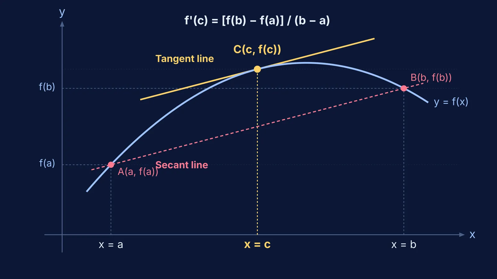
In modern mathematics, the theorem establishes that any well-behaved curve has a tangent parallel to its chord. Formally, let f be a real-valued function that satisfies two conditions:
f is continuous on the closed interval [a, b].
f is differentiable on the open interval (a, b).
Then there exists at least one value c in the open interval (a, b) such that:
f'(c) = [f(b) − f(a)] / (b − a)
The right side of this equation is the slope of the secant line joining the endpoints A(a, f(a)) and B(b, f(b)). The left side is the slope of the tangent line at the point (c, f(c)). The theorem guarantees that at least once between a and b, the tangent runs parallel to the secant.
When you visualize the tangent sliding along the curve until its slope matches the chord, the geometry becomes intuitive. The Fermi Simulation Lab provides interactive simulations for ideas that are easier to see than to read, allowing students to drag interval endpoints and watch the parallel tangent line adjust in real time.
How did Rolle and Cauchy shape the modern textbook proof?
The path from Lagrange's series to the standard proof taught in school classrooms took nearly a century. In 1691, French mathematician Michel Rolle published *Démonstration d'une Méthode pour résoudre les Egalitez de tous les degrez* (MacTutor History of Mathematics). Rolle proved that between any two roots of a polynomial, there lies at least one root of its derivative. Ironically, Rolle was an outspoken opponent of infinitesimal calculus, famously dismissing its methods as "a collection of ingenious fallacies."
In 1823, Augustin-Louis Cauchy published his *Résumé des leçons sur le calcul infinitésimal* (MacTutor History of Mathematics). Cauchy discarded Lagrange's power-series assumption, replacing it with the rigorous limit definition of the derivative. This led to Cauchy's limit-based reformulation and the extended mean value theorem, which relates two functions f(x) and g(x) to prove L'Hôpital's Rule.
The standard textbook proof used today was introduced in 1868 by Pierre-Ossian Bonnet, as recorded in Joseph-Alfred Serret's calculus course. Bonnet constructed an auxiliary function that subtracts the chord from the curve:
g(x) = f(x) − f(a) − [[f(b) − f(a)] / (b − a)] × (x − a)
Because g(a) = 0 and g(b) = 0, g(x) satisfies Rolle's theorem on [a, b]. Differentiating g(x) gives g'(c) = 0, which immediately yields f'(c) = [f(b) − f(a)] / (b − a).
How do you solve an exam problem using the theorem?
Exam problems on Lagrange's Mean Value Theorem typically ask you to verify the conditions on a specified interval and find the value of c.
Worked example: Verify the theorem for f(x) = x³ − 3x on the closed interval [0, 2], and find the value of c.
Check conditions: Because f(x) is a polynomial, it is continuous on [0, 2] and differentiable on (0, 2).
Calculate endpoints: f(0) = 0³ − 3(0) = 0, and f(2) = 2³ − 3(2) = 8 − 6 = 2.
Compute average slope: [f(2) − f(0)] / (2 − 0) = (2 − 0) / 2 = 1.
Solve for c: The derivative is f'(x) = 3x² − 3. Setting f'(c) = 1 gives 3c² − 3 = 1, so 3c² = 4, and c² = 4/3. This yields c = ± 2/√3 ≈ ± 1.155.
Select the valid root: The negative root −2/√3 lies outside the interval. The positive root +2/√3 lies strictly inside the open interval (0, 2), verifying the theorem.
For related problems involving tangent and normal calculations, remember that c must strictly belong to the open interval (a, b), never the endpoints. If you get stuck verifying whether the conditions hold on tricky piecewise or modulus functions, the Fermi Problem Library offers worked problems with a step-by-step solver that explains the reasoning rather than printing an answer.


