

On this page
For centuries, textbooks described the aurora borealis as sunlight reflecting off polar ice or lightning discharging through thin air. Kristian Birkeland, a physics professor in Christiania (now Oslo), realised something far grander was occurring: magnetic compass needles across Europe twitched whenever auroras lit the Arctic sky. Building on William Gilbert's concept that the Earth behaves as a giant magnet, Birkeland proposed in 1896 that sunspots eject beams of cathode rays (electrons) that travel through space, get trapped by Earth's dipole field, and strike atmospheric gases to produce light. He confirmed the link during Arctic expeditions, including the winter of 1899–1900 at the 904-metre-high Haldde observatory and the four-station 1902–1903 campaign (Birkeland, 1908; Egeland and Burke, 2010).
How did the terrella experiment simulate space in a laboratory?
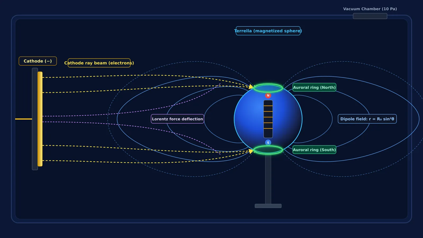
To prove that charged particles could cross a vacuum to create auroras, Birkeland built 17 vacuum chambers between 1896 and 1913, culminating in a 1,000-litre brass-and-glass chamber known as "The Universe" (Lilensten et al., 2013). Inside, he placed a "terrella"—a hollow copper sphere (2.5 cm to 36 cm in diameter) containing an electromagnet that generated fields of roughly 0.5 Tesla. At a chamber pressure of 10 Pa, he fired cathode rays accelerated by 300 V to 1,000 V at 0.1 to 1.0 mA toward the sphere.
Without the magnet, electrons struck the sphere uniformly. The moment current energized the coil, the magnetic field deflected incoming electrons away from the equator and guided them along converging field lines into two bright glowing rings around the poles, reproducing Earth's auroral ovals.
Visualising three-dimensional particle trajectories along curved dipole field lines can be difficult on static paper. The Fermi Simulation Lab provides interactive simulations for ideas that are easier to see than to read, allowing you to manipulate field strengths and particle angles to see how charged particles get guided and trapped.
What is the physics behind charged particle trapping and auroral rings?
The motion follows the Lorentz force F = q(v × B). Because F is always perpendicular to velocity v, it does no mechanical work, leaving kinetic energy constant. The perpendicular component v_perp makes the electron gyrate with Larmor radius r_L = (m v_perp) / (|q| B), producing a helical trajectory of a charged particle in a magnetic field.
As an electron moves toward the poles, the magnetic field B strengthens. Because the first adiabatic invariant μ = (m v_perp²) / (2 B) is conserved, perpendicular energy grows at the expense of parallel motion:
v_parallel² = v₀² − (2 μ B / m)
When v_parallel reaches zero, the electron mirrors back toward space. It precipitates into the atmosphere only if its initial pitch angle α falls inside the loss cone: sin²(α_c) = B_eq / B_iono (Tesema et al., 2020). If an equatorial field B_eq in the plasma sheet (near 10 Earth radii) is 30 nT and the ionospheric field B_iono at 100 km altitude is 50,000 nT:
sin²(α_c) = 30 / 50,000 = 0.0006
sin(α_c) ≈ 0.0245, giving α_c ≈ 1.4°.
Electrons with pitch angles below 1.4° plunge into the thermosphere between 100 km and 150 km, exciting oxygen and nitrogen to emit green (557.7 nm) and red (630.0 nm) auroral light.
When calculating cyclotron radii and pitch-angle mirror points for competitive exams, students often lose track of vector cross products and energy invariants. The Fermi Problem Library features worked problems with a step-by-step solver that explains the reasoning rather than printing an answer, helping you master charged-particle dynamics from first principles.
How were Birkeland currents finally confirmed in space?
For decades, geophysicist Sydney Chapman rejected Birkeland's model, asserting that interplanetary space was a vacuum incapable of carrying electric currents. Birkeland and mathematician Carl Størmer—who spent over 18,000 hours calculating particle trajectories in dipole fields—maintained that currents flowed along magnetic lines (Egeland and Burke, 2010). Swedish physicist Hannes Alfvén later championed the concept, which gained weight once satellite data verified Eugene Parker's mathematical model of the solar wind.
Definitive proof arrived in 1966, when satellite 1963-38C detected transverse magnetic perturbations at 1,100 km altitude (Zmuda et al., 1966). In 1967, W. D. Cummings and A. J. Dessler proved these perturbations were the magnetic signatures of field-aligned currents predicted by Birkeland in 1908 (Cummings and Dessler, 1967). In 1974, Triad satellite data confirmed these conduits carry 1,000,000 to 3,000,000 amperes (Zmuda and Armstrong, 1974). Today, these electric pathways are officially called Birkeland currents, honouring the physicist who first captured the northern lights inside a glass sphere.


