On this page
When you read a modern research paper or an official government survey, you rarely see a single number presented as absolute, unshakeable truth. Instead, estimates are bounded by margins of error. This standard way of reporting scientific and statistical uncertainty was formally introduced by the mathematician Jerzy Neyman. Before his work, there was no universally accepted framework to say exactly how reliable a sample estimate was.
What did Jerzy Neyman invent in 1937?
Jerzy Neyman published his landmark paper, "Outline of a Theory of Statistical Estimation Based on the Classical Theory of Probability," in 1937. At the time, he was a Reader in Statistics at University College, London. Before this foundational work, statisticians often relied entirely on hypothesis testing, which only allowed them to reject or accept a specific, predefined claim.
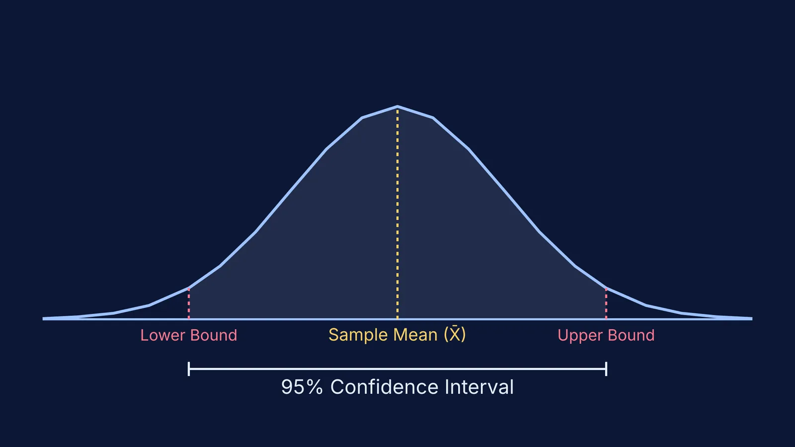
Neyman sought a rigorous mathematical way to estimate an unknown population parameter, such as a mean or a proportion, strictly from a limited sample. He proposed the concept of the confidence interval. A confidence interval provides a continuous range of values that is likely to contain the true parameter. Neyman's approach was firmly rooted in classical, frequentist probability, meaning he viewed the true population parameter as a fixed, unknown constant, while the calculated interval itself was treated as the random variable.
If you are learning these concepts for an exam, mastering the difference between sample statistics and population parameters is essential. The Fermi Problem Library has worked problems with a step-by-step solver that explains the reasoning rather than printing an answer, helping you see how these limits are derived from raw data.
Why do we need a confidence interval in a survey?
We need confidence intervals because it is almost never possible or practical to measure an entire population. Instead, scientists measure a representative sample. Because a sample is only a small subset of the total population, the final calculated result will naturally vary slightly each time you draw a new sample.
Consider a major national demographic survey. The National Family Health Survey (NFHS-5) reported that India's Total Fertility Rate has declined to 2.0 children per woman. This figure is a carefully weighted estimate based on a sample of households across the country. Because the researchers could not literally survey every single household in India, estimates like this are reported with a confidence interval to show their precision.
This range provides an immediate, visual measure of precision. If the confidence interval is very wide, it tells the reader that the estimate has high uncertainty, perhaps because the sample size was too small. If the interval is narrow, the estimate is highly precise and can be trusted for serious policy decisions.
How do you calculate a confidence interval?
Calculating a confidence interval requires three specific pieces of information from your survey or experiment: the sample mean, the sample standard deviation, and the total sample size.
Here is the standard framework for a large sample:
Find the sample mean: This is your best single estimate of the population parameter.
Determine the standard error: Divide the sample standard deviation by the square root of your total sample size. This metric tells you how much the sample mean is expected to fluctuate from the true mean.
Choose a multiplier: Select a mathematical multiplier (often called a z-score) that corresponds to your chosen confidence level.
Calculate the margin of error: Multiply the standard error by the multiplier.
Construct the bounds: Subtract the margin of error from the sample mean to get the lower bound, and add the margin of error to the sample mean to get the upper bound.
For students exploring the mathematical foundations of these rules, you might want to review how foundational changes to data shift these bounds. A related read on how adding to or scaling data changes the mean and variance is How adding to or scaling data changes the mean and variance.
What is the frequentist interpretation of probability?
Neyman's confidence intervals sparked a long and famous philosophical debate in the scientific community, particularly with his contemporary R. A. Fisher. Neyman insisted on a strict frequentist interpretation of probability, which changed how researchers talk about their findings today.
In the frequentist view, a parameter like a true national average is not a random variable; it is a fixed physical fact of the universe. Therefore, you cannot mathematically say "there is a high probability that the true mean is inside this specific interval." Once you calculate the actual interval from your data, the true mean is either inside it or outside it. There is no probability left.
The probability applies strictly to the *procedure* over the long run, before the sample is even drawn. It is a subtle but critical distinction that forms the bedrock of modern statistical reporting and ensures that researchers do not make false promises about their single sample.
If you are preparing for statistics in your board exams, these foundational ideas appear early on. You can read more about how probability is introduced in Probability in Class 10: cards, dice and coins worked step by step. If you find yourself stuck on a tricky concept, Fermi's AI tutor can work out what you already know and build a plan for the session, so you sit down to a clear next step.