On this page
For over a century after Rudolf Clausius introduced entropy in 1865, physics faced a puzzle. According to the Second Law of Thermodynamics and Ludwig Boltzmann's statistical mechanics, isolated systems drift toward maximum disorder, settling into inert equilibrium. Yet nature generates living cells, cyclones, and chemical oscillations. How could complex structures emerge without violating Rudolf Clausius and the idea of entropy?
The Belgian physical chemist Ilya Prigogine resolved this tension by extending thermodynamics to systems operating far from equilibrium. For this theoretical work, Prigogine received the 1977 Nobel Prize in Chemistry as the sole laureate (Nobel Prize). He demonstrated that non-equilibrium states do not merely degrade energy; continuous energy dissipation can create and stabilize macroscopic order.
What are dissipative structures in thermodynamics?
Prigogine first introduced the term "dissipative structures" in 1967 during his address "Structure, Dissipation and Life" and in a foundational paper co-authored with Grégoire Nicolis in the Journal of Chemical Physics. To understand what makes these structures unique, Prigogine distinguished them from equilibrium structures such as salt crystals or diamonds.
An equilibrium structure forms as a closed system cools and minimizes free energy. Once formed, a crystal requires no continuous flow of matter or energy to maintain its rigid lattice. A dissipative structure is the opposite:
It exists exclusively in an open system exchanging mass or energy with its surroundings.
It operates far from thermodynamic equilibrium, where linear relations between forces and fluxes break down.
It maintains its architecture only by continuously dissipating energy into the environment.
If you shut off the incoming flow of energy, a dissipative structure collapses into thermal disorder. In his Nobel lecture on 8 December 1977, titled "Time, Structure and Fluctuations" (Nobel Lecture), Prigogine explained that far from equilibrium, tiny microscopic fluctuations cease to be damped out. Instead, they can cross a critical instability threshold, driving the entire system into a new, organized macroscopic state.
How do systems create order while producing entropy?
Prigogine made this concept mathematically rigorous by splitting the total entropy change (dS) of a system into two distinct components:
dS = d_e S + d_i S
As outlined in Prigogine's Nobel lecture, the term d_i S represents internal entropy production from irreversible processes like friction, diffusion, and chemical reactions. By the Second Law of Thermodynamics, internal entropy production is never negative: d_i S ≥ 0. In an isolated system (d_e S = 0), dS must therefore always be non-negative, driving the system toward maximum disorder.
In an open system, however, the exchange term d_e S can be negative when the system exports heat, matter, or high-entropy byproducts to its environment. When a system reaches a non-equilibrium steady state, its internal state variables remain constant over time (dS = 0). This requires:
d_e S = -d_i S ≤ 0
How does the entropy balance equation work in practice?
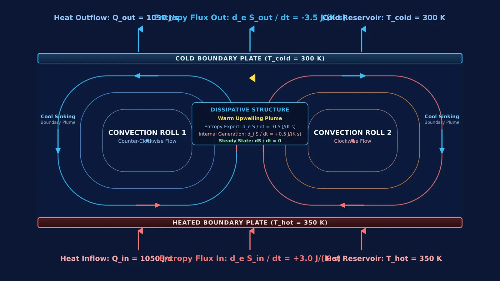
To see how a dissipative structure functions according to dissipative systems theory, consider a shallow fluid layer heated from below in a classical Rayleigh-Bénard convection experiment:
Setup: A fluid layer rests between a heated base at T_hot = 350 K and a cooled top at T_cold = 300 K.
Heat throughput: Steady heat flows through the fluid at Q = 1050 J/s.
Entropy exchange: Heat enters at the base with an entropy flux of d_e S_in / dt = Q / T_hot = 1050 / 350 = +3.0 J/(K·s). Heat exits at the top with an entropy flux of d_e S_out / dt = -Q / T_cold = -1050 / 300 = -3.5 J/(K·s).
Net external flux: Summing both boundaries gives d_e S / dt = 3.0 - 3.5 = -0.5 J/(K·s).
Internal entropy balance: Because steady convection rolls maintain dS/dt = 0, internal entropy production must be d_i S / dt = -d_e S / dt = +0.5 J/(K·s) ≥ 0.
As detailed in Prigogine's Nobel lecture, the surroundings absorb a net positive entropy of +0.5 J/(K·s) every second, ensuring the total entropy of the universe steadily increases. Meanwhile, the fluid layer uses this continuous throughput of energy to organize billions of molecules into synchronized, counter-rotating convection rolls rather than random thermal jiggling.
Where do dissipative structures appear in nature?
Dissipative structures are not rare laboratory curiosities; they represent the primary mechanism of spontaneous self-organization across nature, as detailed in research on dissipative systems:
Rayleigh-Bénard convection: When the temperature difference across a fluid exceeds a critical Rayleigh number, silent conduction gives way to spontaneous hexagonal convection cells.
The Belousov-Zhabotinsky reaction: In 1968, Prigogine and René Lefever developed the Brusselator model to describe autocatalytic chemical networks. Far from equilibrium, chemical concentrations oscillate like a clock or emit expanding concentric rings.
Living cells: Every living cell is an open dissipative structure. By consuming low-entropy nutrients and expelling high-entropy waste heat, cells sustain internal order, membranes, and genetic structures.
How to master thermodynamics with Fermi
Visualizing how energy flows and phase boundaries form is crucial when studying non-equilibrium processes and thermal dynamics. The Simulation Lab provides interactive simulations for the ideas that are easier to see than to read, helping students watch convection patterns and dynamical systems develop in real time.
When working through numerical questions on heat engines, cycle efficiency, and entropy changes, the Fermi Problem Library offers worked problems with a step-by-step solver that explains the reasoning rather than printing an answer.
To connect foundational physical principles across related domains, the Concept Library covers every concept in physics, chemistry, biology, mathematics and computing, each with its own lesson and its place in the map.