

On this page
Why was Heinrich Schwabe searching for an unknown planet?
In 1826, an apothecary in Dessau named Samuel Heinrich Schwabe pointed a small telescope toward the Sun with a singular ambition: he wanted to discover a new planet. At the time, astronomers wondered whether an undetected intra-Mercurial planet—later dubbed Vulcan—circled inside Mercury's orbit. Because any planet so near the Sun was lost in solar glare, the only practical way to spot it was during a transit across the solar disc as a small, round black dot gliding against the bright background.
Schwabe had trained in pharmacy and chemistry in Berlin before managing his family's shop in Dessau for seventeen years until selling it in 1829. Using refracting telescopes with lenses crafted by Joseph von Fraunhofer, he inspected the Sun on every clear morning. To avoid mistaking ordinary sunspots for a transiting planet, Schwabe recorded the count and position of every spot group on every observing day, publishing his method in Astronomische Nachrichten.
How did Heinrich Schwabe discover the sunspot cycle?
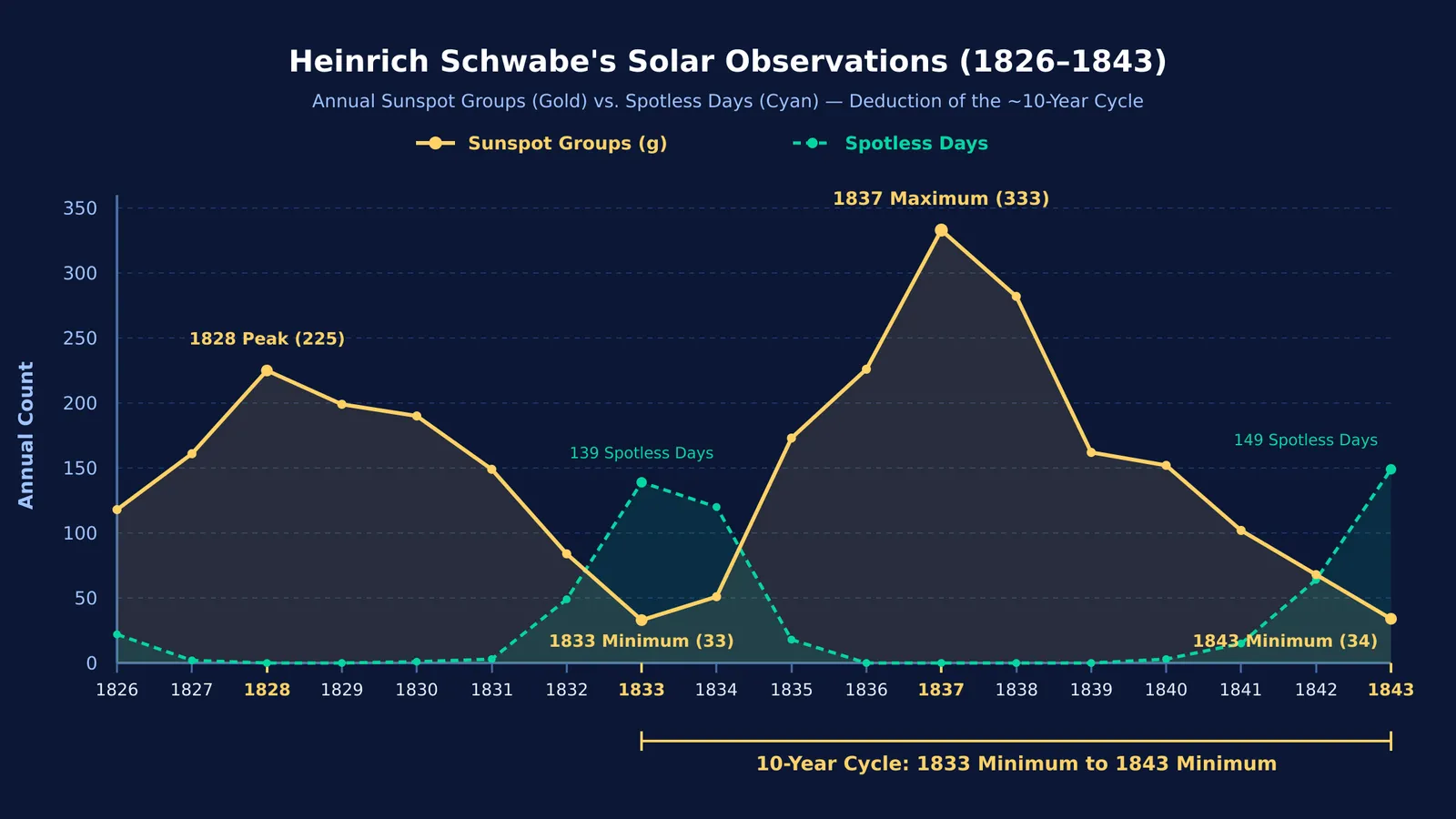
For eighteen years from 1826 through 1843, Schwabe maintained his daily vigil, accumulating records across 4,526 observation days (Schwabe, 1844). He never found the planet, but when he tabulated his annual records in late 1843, an unexpected rhythm emerged from the columns.
In 1828, Schwabe recorded 225 sunspot groups and zero spotless days (Astronomische Nachrichten). By 1833, activity fell to 33 groups and 139 spotless days. Groups surged again to a peak of 333 with zero spotless days in 1837, before dropping back to 34 groups and 149 spotless days in 1843. Comparing the troughs of 1833 and 1843, Schwabe deduced that sunspots follow a period of about 10 years (Schwabe, 1844).
Academic astronomers initially overlooked his four-page report. Recognition came in 1851 when Alexander von Humboldt published Schwabe's table in volume three of *Kosmos*. In 1857, the Royal Astronomical Society awarded Schwabe its Gold Medal. President Manuel J. Johnson remarked: "Twelve years, as I have said, he spent to satisfy himself—six more years to satisfy, and still thirteen more to convince, mankind" (Johnson, 1857). Schwabe reflected with humble humour in a letter published in the society's notices: "I may compare myself to Saul, who went out to seek his father's asses, and found a kingdom."
How is the sunspot cycle calculated today?
Swiss astronomer Rudolf Wolf extended Schwabe's data back to 1610, establishing an average cycle length of 11.1 years (Wolf, 1853), while modern reviews confirm cycles vary between 9 and 14 years (Hathaway, 2015). To standardise counts across observers, Wolf introduced the Relative Sunspot Number:
R = k × (10g + s)
Here g is the number of spot groups, s is the total count of individual spots, and k is an observer correction factor. Groups receive ten times the weight of single spots because new magnetic clusters signify major eruptions of solar activity (Wolf, 1853). For example, if a student observes 4 spot groups with 18 total spots using a standard setup (k = 1.0):
Count groups (g = 4) and total spots (s = 18).
Compute group weighting: 10 × 4 = 40.
Add spots: 40 + 18 = 58.
Scale by observer factor: R = 1.0 × 58 = 58.
Later astronomers deepened these findings: Annie Maunder mapped how spot latitudes drift in Annie Maunder's sunspot butterfly diagram, and George Ellery Hale showed that sunspots carry intense magnetic fields in George Ellery Hale's sunspot magnetism discoveries. When students work through multi-step physics problems involving periodic motion or observational data, the Fermi Problem Library provides worked problems with a step-by-step solver that explains the reasoning rather than printing an answer.
How can students turn daily practice into breakthroughs?
Schwabe discovered the cycle through consistent daily observation rather than sudden inspiration. For students mastering quantitative physics and problem-solving, this systematic logging turns daily practice into real insight:
Track objective counts daily: log problems attempted, errors, and unattempted types instead of vague study hours.
Group mistakes by mechanism: classify errors into conceptual gaps, formula slips, or calculation mistakes.
Review trends across multi-week windows: track accuracy curves over several weeks to spot plateaus and measure retention.
Watch for secondary discoveries: working a hard problem often reveals an algebraic pattern or physical intuition broader than the problem itself.
When abstract concepts like magnetic fields or harmonic oscillations are difficult to picture from text alone, the Fermi Simulation Lab offers interactive simulations for ideas that are easier to see than to read.


