
On this page
An ordinary X-ray squashes the whole body into one flat shadow. CT, computed tomography, gives you slices. The person who made it work in hospitals was not a doctor but an electrical engineer at the British company EMI, Godfrey Hounsfield. This post covers how he got there, the scale he defined, and a small calculation that shows why CT needs many angles.
Who was Godfrey Hounsfield?
Hounsfield was born near Newark, Nottinghamshire, in 1919 and died in 2004, according to his Nobel facts page. In his Nobel autobiography he describes a farm childhood of homemade gliders and water-propelled tar barrels, and a grammar school where he "responded only to physics and mathematics with any ease".
In the Second World War he joined the RAF and became a radar instructor. After the war a grant took him to Faraday House Electrical Engineering College in London. He joined EMI in 1951, and from about 1958 led the team that built the EMIDEC 1100, which he calls the first all-transistor computer constructed in Britain. In 1967, while thinking about automatic pattern recognition, he had the idea that became the EMI scanner.
He shared the 1979 Nobel Prize in Physiology or Medicine with Allan Cormack "for the development of computer assisted tomography". Cormack had published a mathematical method for the problem in 1963, Representation of a function by its line integrals, with some radiological applications.
What was wrong with ordinary X-rays?
In his Nobel lecture, Hounsfield lists three limits:
A flat picture cannot show depth; objects at different depths overlap.
Ordinary X-rays barely tell soft tissues apart; organs like the liver and pancreas are not distinguishable.
They cannot measure the density of each tissue, only the total absorption along the path.
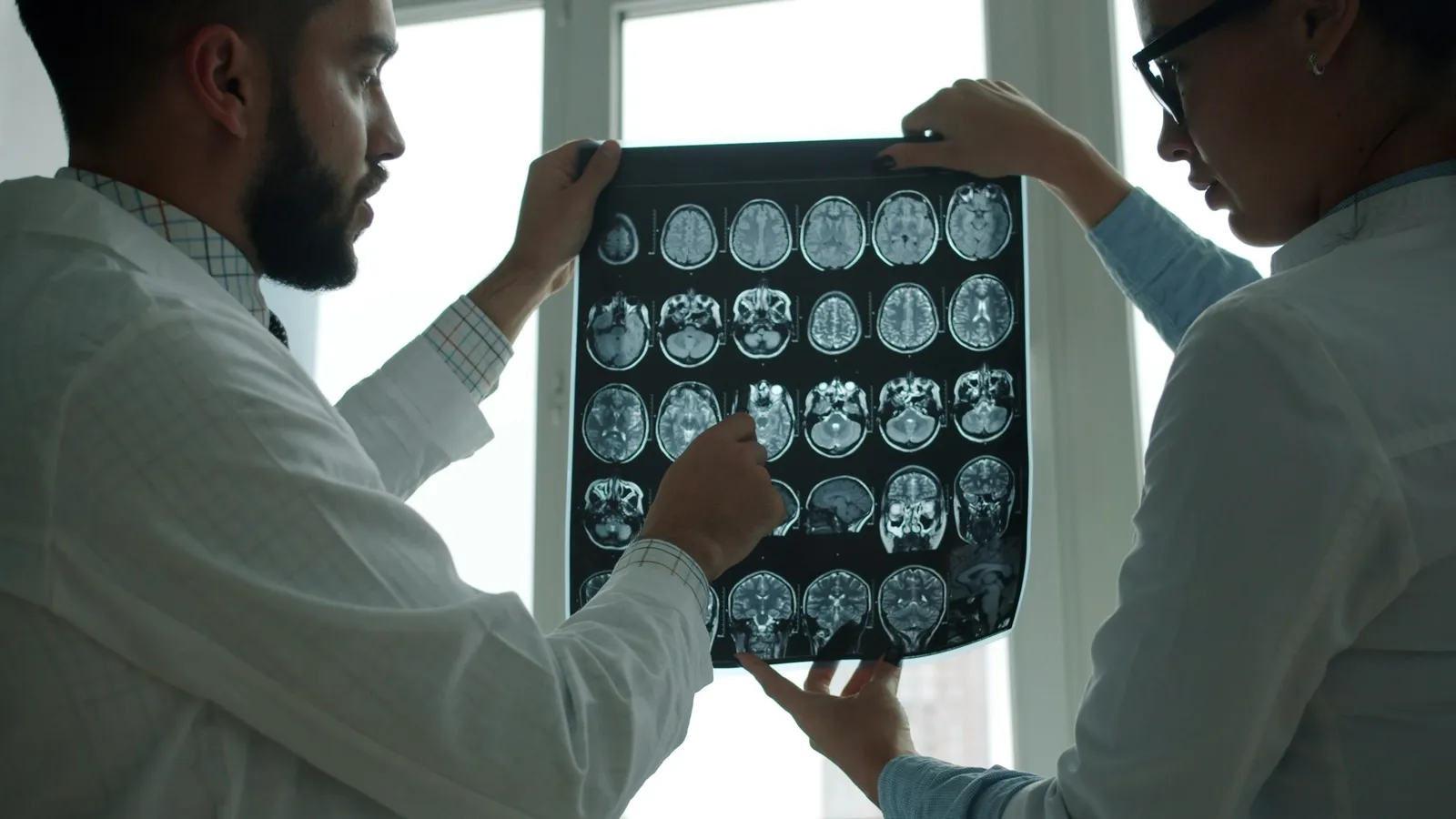
CT instead measures absorption through a slice from hundreds of angles and lets a computer rebuild the slice.
How slow were the first experiments?
The lecture describes the first rig: a gamma-ray source moved along a lathe bed, the object turned 1° after each sweep, and 28,000 readings were punched onto paper tape. A scan took 9 days, and processing took 2 hours on a large computer. Switching to an X-ray tube cut the scan to 9 hours.
Work out the speed-ups:
9 days = 216 hours. 216 ÷ 9 = 24 times faster with the X-ray tube.
9 days for 28,000 readings is 777,600 s ÷ 28,000 ≈ one reading every 28 seconds.
Later body scanners took 18 seconds per picture, and newer ones 3 seconds. From 9 hours (32,400 s) to 18 s is 32,400 ÷ 18 = 1800 times faster.
He tested the method on a preserved human brain, then found the formalin had exaggerated the readings, so he switched to fresh bullock's brains. His autobiography mentions carrying them across London on public transport.
The lecture says the first patient scanned on the clinical prototype at Atkinson Morley's Hospital, London, was a woman with a suspected brain lesion, and the picture "showed clearly in detail a dark circular cyst".
Worked example: why does CT need many angles?
Each beam measures the sum of absorption along its path. The lecture describes the slice as "a mesh of variables" intersected by beams at many angles. Here is the idea with a 2 × 2 grid of unknown squares a, b (top row) and c, d (bottom row). Sample readings, not real data:
Row beams: a + b = 5, c + d = 9
Column beams: a + c = 6, b + d = 8
Try solving. You will find many answers, because the four equations are not independent: the two row sums and the two column sums both add up to 14. Add one diagonal beam:
Diagonal: a + d = 7
Now: b = 5 − a, c = 6 − a, d = 7 − a. Put these into c + d = 9: (6 − a) + (7 − a) = 9, so 13 − 2a = 9 and a = 2. Then b = 3, c = 4, d = 5. Check b + d = 8. It works.
One more angle turned an unsolvable puzzle into a unique answer. A real scanner, the lecture says, takes about a million readings to solve for every small square of the slice.
What is the Hounsfield scale?
The lecture defines the numbers on a CT image: air is −1000, water is 0, and the scale runs about 1000 levels either side of water, up to bone. Add 1000 to a reading and you get a value proportional to true absorption, with air at 0 and water at 1000. That gives:
CT number = 1000 × (μ − μ_water) ÷ μ_water
where μ is the absorption coefficient. With sample values μ_water = 0.200 per cm and a tissue μ = 0.208 per cm, the CT number is 1000 × 0.008 ÷ 0.200 = +40. For air, μ ≈ 0, giving −1000.
Common mistakes: treating CT numbers as densities in kg/m³, and forgetting that water, not air, sets zero.
For where X-rays began, read our post on Wilhelm Röntgen.
What can a student take from Hounsfield's way of working?
Start crude, then speed up. A lathe bed and paper tape were enough to prove the idea.
Distrust a result that looks too good.
Bring skills across fields. Radar and computer design became medical imaging.
Ideas like beams adding up through a grid are easier to follow when you can see them. The Fermi Simulation Lab has interactive simulations for ideas that are easier to see than read.
Next step: make your own 2 × 2 grid with numbers, write the row, column and one diagonal sum, and ask a friend to solve it.