On this page
In May 1852, German physicist and mathematician August Beer published a landmark paper in *Annalen der Physik und Chemie* that reshaped analytical chemistry. Beer showed that light absorption through a solution scales in direct proportion to solute concentration. By uniting his concentration findings with Johann Heinrich Lambert's 1760 rule on path length, Beer's work laid the foundation for the modern Beer-Lambert law: A = εcl. That relation turned color into a quantitative scale, letting chemists, biologists, and astronomers calculate concentrations without destroying their samples.
What did Bouguer and Lambert discover before Beer?
Long before August Beer examined colored liquids, mathematicians investigated why light dims through glass, water, and air. In 1729, French mathematician Pierre Bouguer published *Essai d'optique sur la gradation de la lumière*, founding scientific photometry as described by Encyclopaedia Britannica. Bouguer observed that when a light beam passes through successive slices of equal thickness, each slice absorbs an identical fraction of the light entering it: light intensity falls in a geometric progression.
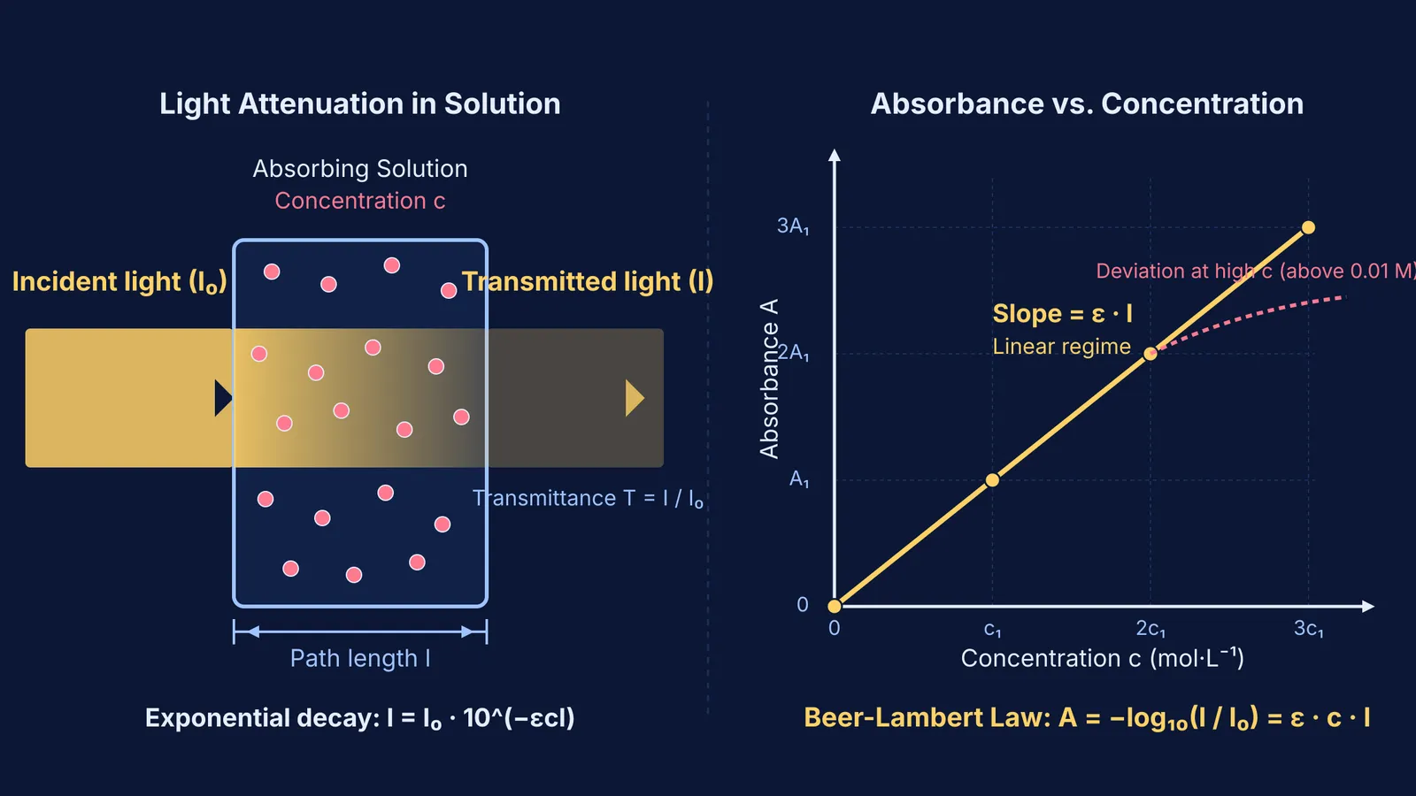
In 1760, Swiss-German polymath Johann Heinrich Lambert formalized Bouguer's discovery in *Photometria*, documented by Encyclopaedia Britannica. Lambert expressed the loss as exponential decay across path length l: transmitted intensity I equals I₀ × 10^(−k·l), where I₀ is incident intensity and k is an absorption coefficient. Yet Bouguer and Lambert examined solid glass or air; neither investigated solutions with variable amounts of dissolved matter.
How did August Beer prove the concentration law in 1852?
Working at the University of Bonn, August Beer tested whether light absorption in solutions depended on chemical concentration. In his 1852 paper, *"Bestimmung der Absorption des rothen Lichts in farbigen Flüssigkeiten"*, published in Annalen der Physik und Chemie, Beer built an optical bench with an adjustable liquid cell and red-filtered light to study aqueous solutions of salts like copper sulfate.
Beer observed that halving the solution's concentration while doubling the cell's path length left light transmission unchanged. As chemists Heinz G. Pfeiffer and Herman A. Liebhafsky noted in the Journal of Chemical Education, absorption depends on the total count of absorbing molecules in the beam path. The IUPAC Compendium of Chemical Terminology defines the combined Beer-Lambert-Bouguer law: decadic absorbance A of monochromatic light in a homogeneous medium is proportional to path length l and concentration c:
A = −log₁₀(I / I₀) = ε × c × l
Here, A is dimensionless absorbance, I / I₀ is transmittance T, c is molar concentration in mol·L⁻¹, l is path length in cm, and ε is molar absorptivity in L·mol⁻¹·cm⁻¹.
Students exploring wave behavior and optics can use the Fermi Simulation Lab, which provides interactive simulations for ideas that are easier to see than to read.
How do you calculate concentration using Beer's law?
Beer's law allows direct calculation of unknown concentrations because absorbance scales linearly with molarity. As Donald F. Swinehart outlined in the Journal of Chemical Education, converting transmission to a decadic absorbance scale linearizes the relationship with solute concentration for quantitative spectrophotometry. When titrating oxalic acid with potassium permanganate or verifying spectrophotometer data, you can determine concentration in three steps:
Zero the instrument: Insert a solvent blank cuvette to calibrate 100% transmittance (A = 0.000).
Measure transmittance: Place the sample in a 1.00 cm cuvette and record transmitted intensity I relative to incident intensity I₀.
Solve for molarity: Calculate A = −log₁₀(I / I₀) and divide by ε × l.
Suppose a student tests aqueous copper(II) sulfate in a 1.00 cm cuvette at 810 nm, where ε is 12.0 L·mol⁻¹·cm⁻¹. The detector reads 25.0% transmission (T = 0.250).
Absorbance: A = −log₁₀(0.250) = log₁₀(4.00) ≈ 0.602.
Concentration: c = A / (ε × l) = 0.602 / (12.0 L·mol⁻¹·cm⁻¹ × 1.00 cm) = 0.0502 mol·L⁻¹ (50.2 mmol·L⁻¹).
When preparing standard dilutions, our guide to mixing and diluting solutions to calculate molarity details the volumetric calculations. For multi-step practice, the Fermi Problem Library has worked problems with a step-by-step solver that explains the reasoning rather than printing an answer.
When does the Beer-Lambert law break down?
Beer's law is an ideal limiting relation that bends under specific conditions. As Thomas G. Mayerhöfer and colleagues analyzed in ChemPhysChem, both electromagnetic wave effects and intermolecular interactions cause real solutions to deviate from ideal linearity:
High solute concentration: Above roughly 0.01 mol·L⁻¹, electrostatic interactions between nearby solute ions perturb electron clouds, shifting the absorption peak and changing ε. High concentrations also alter the bulk refractive index.
Chemical equilibrium shifts: If absorbing molecules associate or dissociate, the chromophore concentration changes nonlinearly. For instance, dichromate in water shifts between orange Cr₂O₇²⁻ and yellow CrO₄²⁻ based on pH and dilution.
Polychromatic light: If incident light contains a range of wavelengths where ε varies, or if stray light reaches the detector, the absorbance curve flattens downward.
Connecting chemical concentrations to light absorption echoes Gustav Kirchhoff's work on spectroscopy. The Fermi Concept Library covers every concept in physics, chemistry, biology, mathematics and computing, each with its own lesson and its place in the map.