

On this page
Before 1882, measuring electric current was a delicate and frustrating task. The standard instrument in laboratories was the moving-magnet galvanometer, such as the tangent galvanometer or the Kelvin astatic galvanometer. These devices used a large, fixed coil of wire and a tiny, suspended magnetic needle. When current flowed through the fixed coil, it created a magnetic field that deflected the needle.
But this design had a critical flaw: the magnetic needle was highly susceptible to outside forces. The Earth's magnetic field and any nearby iron objects constantly interfered with the reading. The instrument had to be carefully aligned with magnetic north before every use, and even then, vibrations could throw off the measurement. Furthermore, its scale was non-linear, meaning the markings were unevenly spaced, which made calculations tedious and prone to error.
How does a moving coil galvanometer work?
In 1882, the French physician and physicist Jacques-Arsène d'Arsonval worked with the engineer Marcel Deprez to turn the design inside out. Instead of a moving magnet, they used a strong, stationary horseshoe magnet. Between its poles, they suspended a light coil of fine wire.
This solved the interference problem immediately. Because the instrument's internal permanent magnet was so strong, the weak magnetic field of the Earth could no longer disturb the readings. The d'Arsonval-Deprez design was highly sensitive, detecting currents as small as ten microamperes (10⁻⁵ A).
Why is a radial magnetic field used in a moving coil galvanometer?
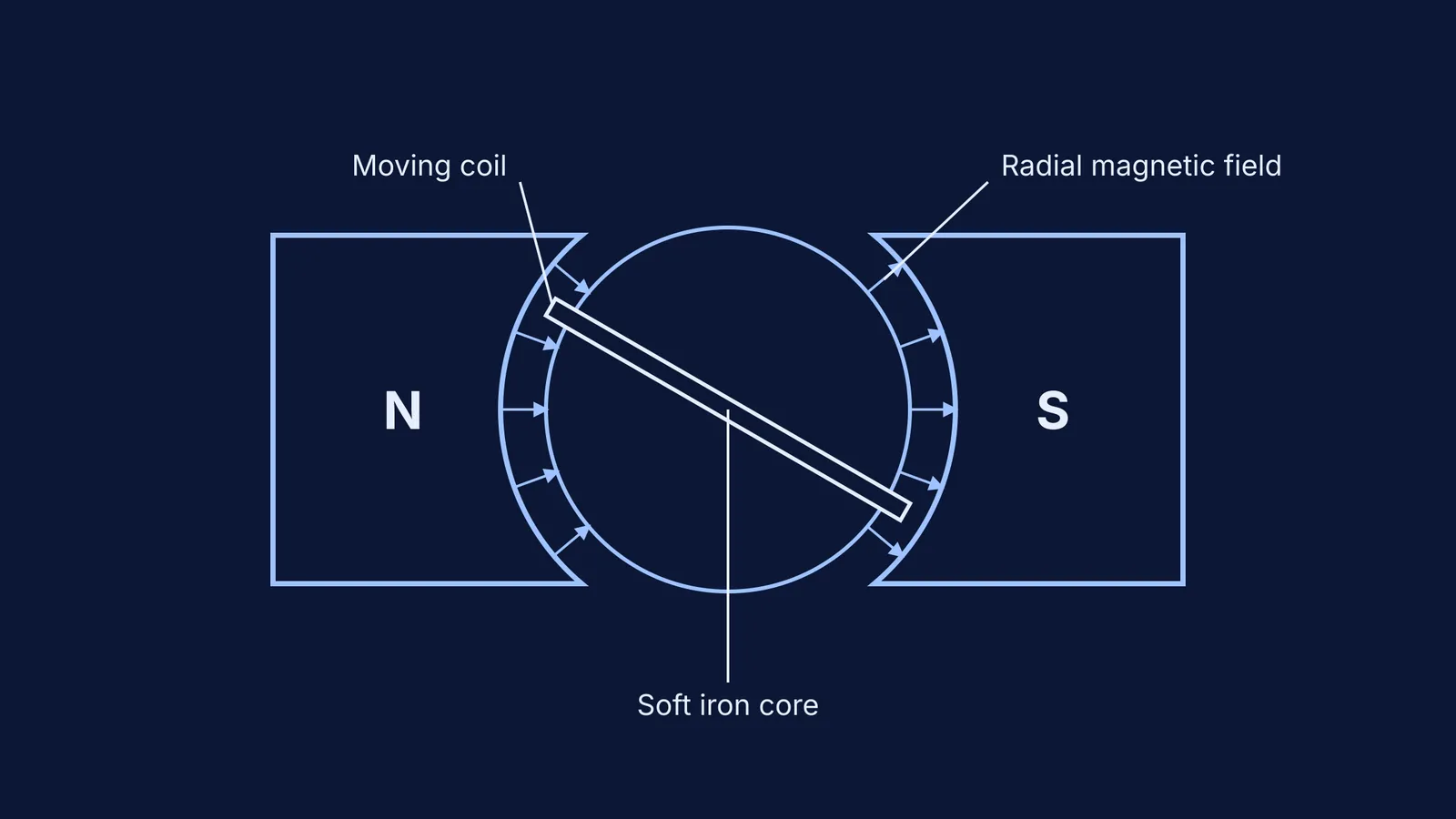
The most important innovation in the d'Arsonval design was its linearity. To make the scale uniform, the magnetic field had to be at right angles to the coil at all times.
D'Arsonval and Deprez achieved this by carving the magnet's poles into concave curves and placing a soft iron cylinder between them. This shaped the magnetic field lines so they radiated outwards like the spokes of a wheel. No matter how the coil turned, its sides always cut the magnetic field lines perpendicularly (θ = 90°).
The torque (τ) on a coil of N turns, area A, carrying current I in a magnetic field B is τ = NIAB sin θ. With a radial field, sin θ = 1, so the torque is simply τ = NIAB. This constant twisting force is balanced by the restoring torque of the suspension (kα, where k is the torsional constant and α is the angle of deflection). Setting them equal gives I = (k / NAB) α. Because the current is directly proportional to the deflection, the scale can be marked with evenly spaced lines.
If you get stuck trying to remember which terms belong in the torque equation, the Fermi Problem Library has worked problems with a step-by-step solver that explains the reasoning rather than printing an answer.
What are the Weston improvements and dead-beat damping?
The 1882 design was a major advance, but the fine suspension wires—often made of delicate phosphor bronze—were fragile and prone to snapping. In 1888, the engineer Edward Weston refined the d'Arsonval galvanometer into the rugged instrument we use today. Weston replaced the suspension wires with jewelled pivots and delicate spiral springs, similar to the hairspring in a mechanical watch.
Weston also improved the damping. When the coil swings in a sensitive instrument, you do not want the pointer to bounce back and forth for several seconds before settling. By winding the copper coil on a light, conductive aluminium frame, the motion induces eddy currents in the frame. According to Lenz's law, these induced currents oppose the motion that created them, bringing the pointer smoothly to a halt without oscillation. This self-braking feature is known as "dead-beat" damping.
How to master galvanometer problems
The moving-coil galvanometer is a core topic in high school physics and competitive engineering exams like the JEE. To master it, you need to understand both its mechanical balance and its electrical behaviour in a circuit.
Here is a checklist for your exam preparation:
Learn the torque derivation: Be ready to derive τ = NIAB from the force on a current-carrying wire.
Understand the geometry: Know why the soft iron core and concave pole pieces are essential for a linear scale.
Practise circuit conversions: Practise converting the galvanometer into an ammeter and voltmeter using Ohm's law and Kirchhoff's rules.
Study the practicals: Know how to find the Galvanometer resistance and figure of merit by half deflection in the lab.
Once you grasp the principle of the moving coil, you will find it easier to tackle related topics, such as the Moving coil galvanometer: converting it to an ammeter and voltmeter and even the fundamental physics discussed in André-Marie Ampère and the force between two currents.


