On this page
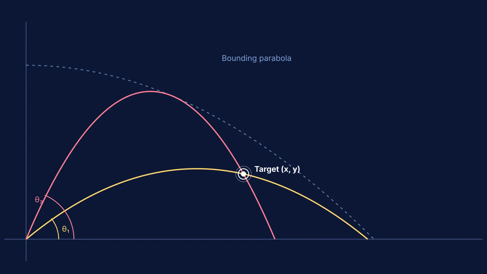
If you throw a ball at a target, there are usually two ways to hit it: a fast, flat throw or a slow, high lob. In physics, this is a mathematical certainty. For any reachable target in projectile motion, there are exactly two angles of projection that will hit the same coordinate (x, y) for a given launch speed, unless the target is at the very limit of the throw.
To prove this, we do not need to guess. We can reshape the standard equation of motion into a quadratic equation in tan θ, revealing the exact angles and the physical limits of the throw.
The trajectory equation as a quadratic in tan θ
The standard equation of trajectory of a projectile links the vertical position y to the horizontal position x, the initial velocity u, and the launch angle θ:
y = x tan θ − gx² / (2u² cos² θ)
This form is useful if you already know the launch angle and simply want to map the flight path. But if the target coordinates (x, y) and the launch speed u are fixed by the problem, and you want to find the required angle θ, the cos² θ term sitting in the denominator makes the algebra difficult to isolate.
We can rewrite it using the fundamental trigonometric identity 1 / cos² θ = sec² θ = 1 + tan² θ. Substituting this relationship back into the trajectory equation removes the cosine term entirely and gives:
y = x tan θ − (gx² / 2u²) (1 + tan² θ)
Now, let's rearrange this to group the terms by powers of tan θ:
(gx² / 2u²) tan² θ − x tan θ + (y + gx² / 2u²) = 0
This is a standard quadratic equation in the form az² + bz + c = 0, where our variable z is tan θ.
How do you find the two angles of projection?
Because it is a quadratic equation, solving for tan θ will generally yield two roots. This mathematical result explains the physical reality: there are two valid trajectories to the target.
The smaller root: This gives a smaller angle θ₁. It corresponds to the "low trajectory"—a flatter, faster path that reaches the target in less time.
The larger root: This gives a larger angle θ₂. It corresponds to the "high trajectory"—a steeper, lofted path that stays in the air longer.
If you struggle with the algebraic rearrangements required for 2D kinematics, the Concept Library breaks down the trajectory equation step-by-step. Fermi's AI tutor can walk you through the substitutions and show you how to apply the quadratic formula without losing track of the physics.
What is the condition for any solution?
In a quadratic equation az² + bz + c = 0, real solutions only exist if the discriminant (b² − 4ac) is greater than or equal to zero.
If we calculate the discriminant for our trajectory quadratic and set b² − 4ac ≥ 0, we get:
x² − 4(gx² / 2u²)(y + gx² / 2u²) ≥ 0
With some simplification, this inequality rearranges to an upper limit for the height y at a given distance x:
y ≤ u² / 2g − gx² / 2u²
This curve is known as the bounding parabola or the envelope of trajectories. It represents the absolute boundary of space the projectile can reach with speed u.
Inside the envelope (b² − 4ac > 0): The target is reachable. There are exactly two launch angles to hit it.
On the envelope (b² − 4ac = 0): The target is at the extreme limit of the projectile's range. The two angles merge into one optimal angle.
Outside the envelope (b² − 4ac < 0): The target is too far or too high. No real angle exists that can hit it; you need a faster launch speed.
Understanding this boundary is crucial for harder mechanics problems, such as determining whether two projectiles will collide midair or calculating the safe zone around an explosion. When setting up these problems, start by drawing the envelope of trajectories to quickly visualise what is possible. If you are preparing for exams like the JEE, testing boundaries and interpreting discriminant conditions is a highly examinable skill. You can practice applying this specific condition in the Fermi Problem Library, where the solver will help you interpret what a negative discriminant means for your specific target coordinates.