

On this page
What is a moving average in time series analysis?
A time series is a sequence of observations recorded at regular intervals, such as annual crop yields, monthly revenue, or daily temperatures. Observed data rarely follows a straight line; it combines secular trend, seasonal cycles, economic waves, and random noise. In statistical analysis, these forces are separated through time series decomposition. As outlined in the CBSE Applied Mathematics curriculum, the additive model expresses an observed value y as y = T + S + C + I, where T is the secular trend, S is seasonal variation, C is cyclical variation, and I is irregular variation.
The secular trend shows the general direction of the data, but short-term fluctuations often conceal it. A moving average smooths the series so the trend emerges clearly. Rather than calculating a single overall mean, it computes the arithmetic mean of a rolling subset of consecutive observations. As the window advances by one period, the oldest observation drops out and the newest enters the sum.
Moving averages date to 1901, when statistician R. H. Hooker published a study on marriage rates and trade cycles in the Journal of the Royal Statistical Society. Hooker showed that rolling averages dampen oscillations without forcing data into a rigid linear mold. How rolling subsets redistribute variation connects directly to mean, variance and standard deviation.
How do you calculate a three-year moving average?
An odd-period moving average uses an odd window width (m = 2k + 1), such as m = 3 (where k = 1). The key advantage is geometric symmetry: the mean of three consecutive numbers aligns naturally with the middle time unit. In guidelines from the NIST Information Technology Laboratory, moving averages advance a fixed window across time so each smoothed value represents the local central tendency.
To calculate a three-year moving average:
Sum three consecutive values: Total_t = y_{t-1} + y_t + y_{t+1}.
Divide by 3: T_t = Total_t / 3.
Place the value against the middle year (time t), then advance the window by one year.
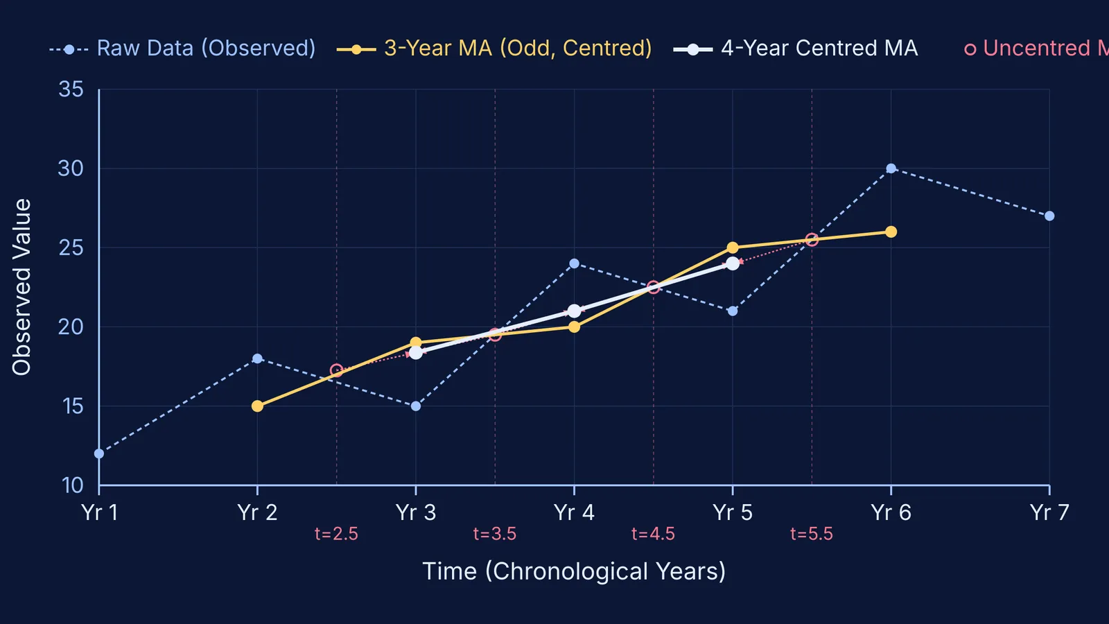
Consider sales across six consecutive years: Year 1 = 12, Year 2 = 18, Year 3 = 15, Year 4 = 24, Year 5 = 21, Year 6 = 30.
Year 2: (12 + 18 + 15) / 3 = 45 / 3 = 15.0.
Year 3: (18 + 15 + 24) / 3 = 57 / 3 = 19.0.
Year 4: (15 + 24 + 21) / 3 = 60 / 3 = 20.0.
Year 5: (24 + 21 + 30) / 3 = 75 / 3 = 25.0.
No moving average exists for Year 1 or Year 6. Because the window requires an adjacent value on each side, an odd window of width m loses k = (m - 1) / 2 points at each boundary, or m - 1 observations in total.
Why do even-period moving averages require centring?
When the averaging period is even, such as four years or four quarters, an alignment problem arises. According to the NIST Engineering Statistics Handbook, the mean of an even number of observations falls at the temporal midpoint between consecutive periods. For times 1, 2, 3, and 4, the midpoint is (1 + 2 + 3 + 4) / 4 = 2.5, landing halfway between Year 2 and Year 3.
To restore chronological alignment, statisticians apply centring. A centered moving average eliminates phase lag by taking a two-period average of adjacent even-period moving averages. Averaging the midpoint between Years 2 and 3 (t = 2.5) with that between Years 3 and 4 (t = 3.5) gives (2.5 + 3.5) / 2 = 3.0, aligning with Year 3.
You can compute this in two ways:
Two-step averaging: Calculate four-year moving averages between years, then take the mean of each adjacent pair.
Centred total division: Add adjacent pairs of four-year totals to form an eight-period total, and divide by 8.
Centring converts an unweighted four-term average into a symmetric five-term weighted average: T_t = (y_{t-2} + 2y_{t-1} + 2y_t + 2y_{t+1} + y_{t+2}) / 8. The inner three observations receive double the weight of the two boundary points. Centring an even window of length m loses m / 2 observations at each end. Exploring how adding or scaling data changes the mean and variance shows how linear combinations alter dispersion.
When working through multi-step statistical derivations, verifying intermediate totals helps catch arithmetic slips early. The Fermi Problem Library has worked problems with a step-by-step solver that explains the reasoning rather than printing an answer.
How does moving average smoothing reveal the secular trend?
The main purpose of calculating moving averages is to eliminate rhythmic fluctuations that obscure long-term trajectories. As outlined in the CBSE Applied Mathematics guidelines, choosing a window equal to the seasonal cycle length (such as m = 4 for quarterly data) ensures that each sum contains exactly one observation from each season. Peaks and troughs cancel out, removing seasonal oscillation from the trend estimate.
Selecting window width balances noise reduction against boundary data loss. A wider window produces a smoother curve, but it blunts sharp turning points and leaves larger gaps at both ends of the series. Plotting the raw line alongside the smoothed moving average provides clear visual intuition, similar to techniques used for reading graphs accurately.
Unlike least-squares lines, moving averages adapt to changing curves without imposing a rigid formula. However, because they cannot compute values past boundary observations, they cannot forecast future periods directly on their own. For students building a deeper foundation across quantitative methods, the Fermi Concept Library covers every concept in physics, chemistry, biology, mathematics and computing, each with its own lesson and its place in the map.


