On this page
When solving linear programming problems in Class 12 maths, you usually expect one clear winner: a single corner point that gives the maximum profit or minimum cost. But sometimes, the math leads to a tie between two vertices.
Graphing these regions uses the same skills you built when studying linear inequalities in Class 11, but finding the optimal solution requires testing the corners. Here is how to know when you have found an infinite number of solutions.
Why do some LPPs have multiple optimal solutions?
The corner point method states that an optimal value must occur at a vertex of the feasible region. But what happens when two vertices tie for the best value?
According to the NCERT textbook, if two corner points of the feasible region are optimal solutions of the same type, then any point on the line segment joining these two points is also an optimal solution (NCERT).
Geometrically, this means your objective function line is exactly parallel to one of the bounding constraints. When you slide the objective function across the graph to maximize or minimize it, it does not just touch a single vertex before leaving the feasible region; it stops flush against an entire edge. Every point on that edge satisfies the constraints and gives the exact same optimal value.
What is a worked example of an LPP with infinite solutions?
Let's set up a standard maximization problem to see how this looks in practice.
Objective: Maximize Z = 3x + 4y
Subject to the constraints:
x + y ≤ 35
3x + 4y ≤ 120
x ≥ 0, y ≥ 0
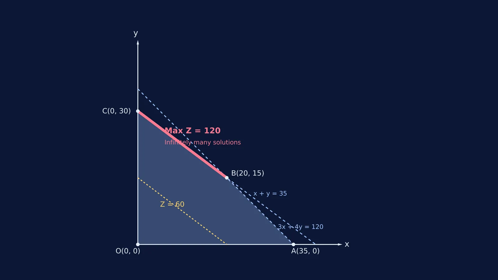
First, we find the corners of the feasible region by plotting the lines and finding their intersections. The intersection of x + y = 35 and 3x + 4y = 120 is the point (20, 15).
The corner points of our feasible region are (0, 0), (35, 0), (20, 15) and (0, 30). Now, we evaluate the objective function Z = 3x + 4y at each point:
At (0, 0): Z = 3(0) + 4(0) = 0
At (35, 0): Z = 3(35) + 4(0) = 105
At (20, 15): Z = 3(20) + 4(15) = 120
At (0, 30): Z = 3(0) + 4(30) = 120
The maximum value is 120, and it occurs at both C(0, 30) and B(20, 15). Because these two points are adjacent corners connected by the constraint line 3x + 4y = 120, every single coordinate on the segment between them will also give Z = 120. For example, the midpoint (10, 22.5) gives 3(10) + 4(22.5) = 30 + 90 = 120.
How do you spot this in an exam?
You can often predict multiple optimal solutions before you even draw the graph. Look at the coefficients of x and y in your objective function and compare them to your constraints.
In our example, the objective Z = 3x + 4y has the exact same coefficients as the constraint 3x + 4y ≤ 120. When you see parallel structures like this, or coefficients that are exact multiples (such as Z = 6x + 8y alongside a 3x + 4y ≤ 120 constraint), expect multiple solutions if that constraint ends up bounding the optimal side of your feasible region.
If you find yourself getting stuck while finding vertices or graphing complex bounds like equations and inequalities with modulus, the Fermi Problem Library has worked problems with a step-by-step solver that explains the reasoning rather than printing an answer. When you bring a problem set to Fermi, the AI tutor builds a plan for the session and teaches through it—drawing the figure and checking understanding as it goes.
A checklist for infinite solutions
When stating your final answer, run through these three checks to ensure you get full marks:
Did you test every vertex? Ensure you haven't missed a corner point that might give a higher value.
Are the tied points adjacent? The two points must be connected by an edge of the feasible region.
Did you write the conclusion clearly? Do not just list the two points. State explicitly: "The maximum value is 120, which occurs at all points on the line segment joining (0, 30) and (20, 15)."