On this page
When you collect raw numerical data—such as examination marks across a classroom or daily temperatures over several weeks—the numbers arrive unorganised. Looking at an unordered list gives little immediate insight into how values cluster or spread. According to NCERT's official textbook curriculum, condensing raw observations into a grouped frequency distribution table reveals patterns, peaks, and ranges that are invisible in an unorganised list.
Constructing these tables accurately requires mastering four connected concepts: class limits, class boundaries, class size, and class marks.
What are class limits, class size, and class marks in Class 9?
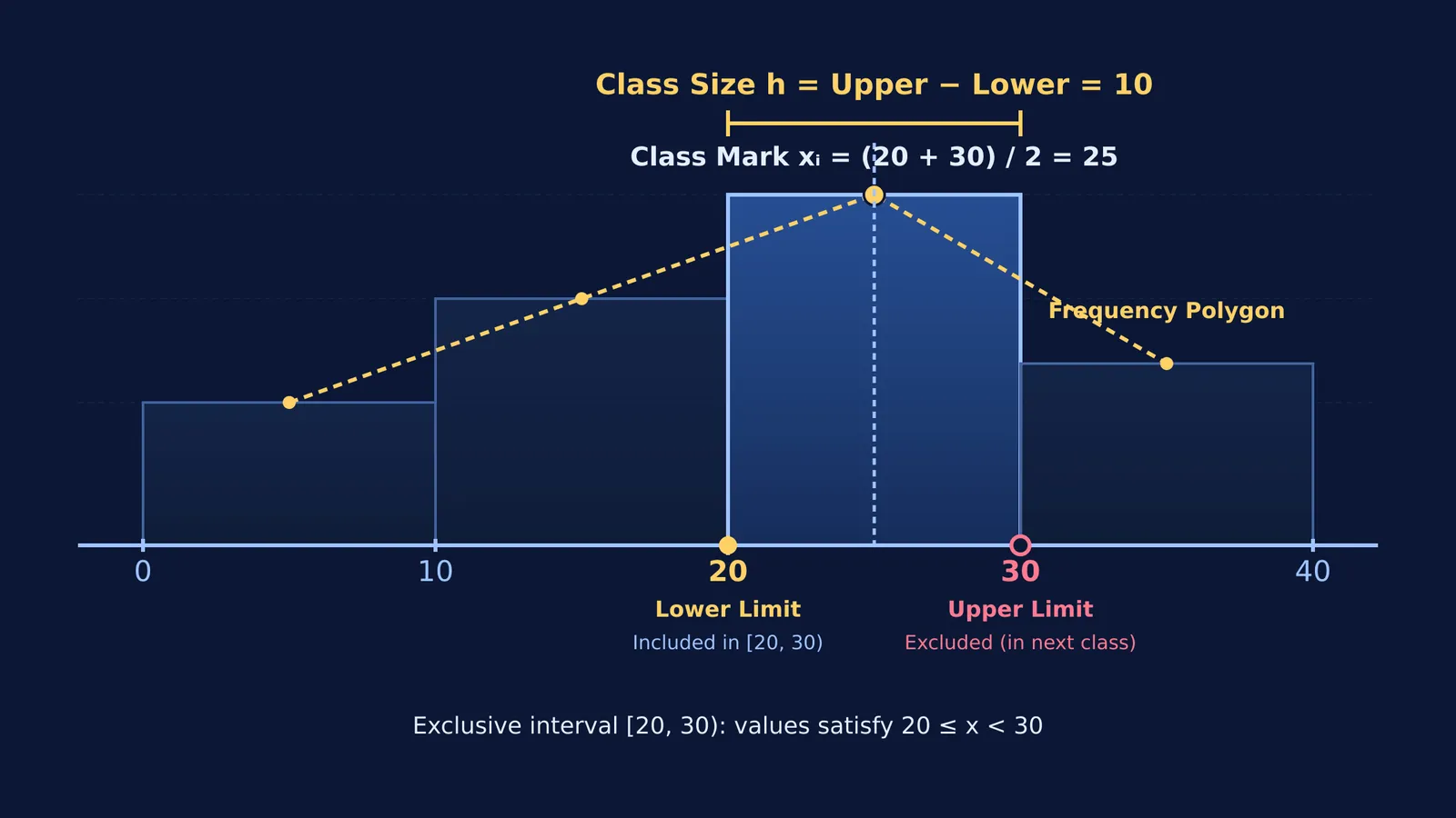
A class interval is a defined band of values used to sort raw numbers. Each interval is framed by two terminal values known as class limits. The smaller value is the lower class limit, and the larger value is the upper class limit. For instance, in the interval 20–30, the lower limit is 20 and the upper limit is 30.
The class size, or class width (denoted by h), measures the breadth of the interval. For continuous groups:
Class size h = Upper class limit − Lower class limit
For 20–30, the class size is 30 − 20 = 10.
The class mark (denoted by xᵢ) is the central value or midpoint of the interval:
Class mark xᵢ = (Upper class limit + Lower class limit) ÷ 2
For 20–30, the class mark is (20 + 30) ÷ 2 = 25. If all intervals have equal width, the difference between consecutive class marks equals the class size h.
The CBSE secondary curriculum for 2024-25 assigns 6 marks to the Statistics unit, emphasizing histograms and frequency polygons. In both representations, class marks provide the horizontal coordinates where frequencies are plotted.
How do you convert inclusive intervals to continuous boundaries?
Grouped intervals appear in two formats:
Exclusive (continuous) form: The upper limit of one class equals the lower limit of the next, such as 10–20, 20–30, and 30–40.
Inclusive (discontinuous) form: A gap exists between successive intervals, such as 11–20, 21–30, and 31–40.
In exclusive intervals, an observation matching a boundary value belongs to the higher class by universal convention. A score of 20 is placed in 20–30, never in 10–20.
When data is arranged in inclusive form, drawing a histogram requires converting limits into continuous class boundaries:
Find the gap d between the lower limit of a class and the upper limit of the preceding class (for 11–20 and 21–30, d = 21 − 20 = 1).
Divide this gap by 2: d ÷ 2 = 0.5.
Subtract 0.5 from every lower class limit to find the lower boundary.
Add 0.5 to every upper class limit to find the upper boundary.
This adjustment converts 11–20 into 10.5–20.5, and 21–30 into 20.5–30.5. Both formats yield the identical class mark: (11 + 20) ÷ 2 = 15.5, and (10.5 + 20.5) ÷ 2 = 15.5.
How do you build a grouped frequency table from raw data?
To build a grouped frequency table systematically, follow five steps:
Determine the range: Calculate the difference between the maximum and minimum observations.
Choose the number of classes: Typically 5 to 10 intervals of uniform width.
Calculate class width: Divide the range by the number of classes and round to a convenient integer.
Write intervals: Begin at or just below the minimum observation.
Tally frequencies: Count each observation into its interval and sum the tallies.
Consider twenty examination scores: 12, 14, 16, 18, 19, 22, 23, 25, 27, 28, 29, 30, 31, 33, 35, 36, 38, 41, 44, 47.
Range: Maximum 47 − Minimum 12 = 35.
Class width of 10 gives four intervals: 10–20, 20–30, 30–40, and 40–50.
Tallying the scores:
10–20: 12, 14, 16, 18, 19 (Frequency = 5; Class mark = 15)
20–30: 22, 23, 25, 27, 28, 29 (Frequency = 6; Class mark = 25)
30–40: 30, 31, 33, 35, 36, 38 (Frequency = 6; Class mark = 35)
40–50: 41, 44, 47 (Frequency = 3; Class mark = 45)
The sum of frequencies is 5 + 6 + 6 + 3 = 20, matching the dataset count. Score 30 falls into 30–40 under the exclusive rule. For graphical follow-ups, see our Class 9 statistics guide on weighted averages and bar charts and explore how origin and scale transformations affect mean and variance.
Why does mastering grouped data structure speed up secondary maths?
Organizing data into grouped tables builds procedural fluency that prevents errors in higher grades. Educational research demonstrates why structured methods succeed: Fred Paas's 1992 study in the Journal of Educational Psychology showed that studying worked examples in statistics reduced subjective cognitive load on a 9-point rating scale and led to superior skill transfer compared to conventional problem-solving.
In Class 10, calculating the mean, median, and mode relies entirely on this grouped foundation, as shown in our guide to Class 10 grouped data methods for mean, median, and mode. The Fermi Problem Library provides worked problems with a step-by-step solver that explains the reasoning rather than printing an answer, helping you verify interval boundaries and tallies.
To see how class midpoints connect to broader concepts, the Fermi Concept Library maps every concept in mathematics, helping you trace how class marks become coordinates for frequency polygons.