On this page
When working through data distributions, histograms are the standard way to picture grouped frequencies. But what if you want to compare two different datasets on the same axes? Two overlapping histograms quickly become a cluttered mess of intersecting bars. A frequency polygon solves this by turning those bulky bars into a single, clean line.
Here is how to draw a frequency polygon from a histogram, why the graph must always be closed, and how to construct one directly from a frequency table.
What is a frequency polygon?
A frequency polygon is a line graph representing a continuous frequency distribution by joining the midpoints of a histogram's bars. Unlike a bar chart, which focuses on discrete categories, a frequency polygon shows the shape of continuous data—much like a curve.
Because it removes the rectangular bars, a frequency polygon is the ideal way to compare two or more sets of data (like the exam marks of two different classrooms) on a single set of axes.
If you are trying to picture why distributions matter or how to visualise continuous functions, the Fermi Concept Library holds lessons on statistics and graphical representations to help you build the intuition behind the formulas.
How to draw a frequency polygon from a histogram?
If you already have a histogram drawn on graph paper, turning it into a frequency polygon takes just three steps.
Find the midpoints: Mark the exact centre point of the upper horizontal line of each rectangular bar.
Join the dots: Use a ruler to connect these midpoints in order, from the lowest class interval to the highest, with straight line segments.
Close the polygon: A frequency polygon must always be a closed geometric figure. To do this, add a hypothetical class interval at the beginning and the end of your histogram, mark their midpoints on the horizontal axis (at zero frequency), and connect your line to them.
Why must it be closed? Because the total area bounded by a frequency polygon and the horizontal axis must remain exactly equal to the total area of the original histogram.
Why do we add zero-frequency classes at both ends?
The most common mistake students make is leaving their frequency polygon "hanging" in mid-air at the first and last data points.
According to standard graphing rules, you must assume a hypothetical class interval immediately preceding your first actual class, and another one immediately following your last class. Both of these hypothetical intervals are assigned a frequency of 0.
If your data starts at 0 (for example, the first class is 0 to 10), the preceding hypothetical class becomes −10 to 0. Its midpoint is −5. You must plot the point (−5, 0) on the x-axis and connect your first histogram midpoint to it, even if a negative value is physically impossible in the real world. This is a mathematical requirement to complete the polygon's area, not a literal data point.
If you get stuck trying to remember whether to subtract or add intervals in an exam, the Fermi Problem Library has step-by-step solvers that explain the reasoning behind class limits rather than just giving you the final graph.
How to draw a frequency polygon without a histogram?
You do not actually need to draw the rectangular bars to find your points. You can draw a frequency polygon directly from a grouped frequency table by calculating the "class mark" for each interval.
The class mark is simply the midpoint of the class interval. You calculate it with a straightforward formula: Class Mark = (Upper Limit + Lower Limit) / 2
A worked example
Suppose you are given a frequency distribution of weights in kilograms and asked to draw a frequency polygon directly. Here is the step-by-step plan:
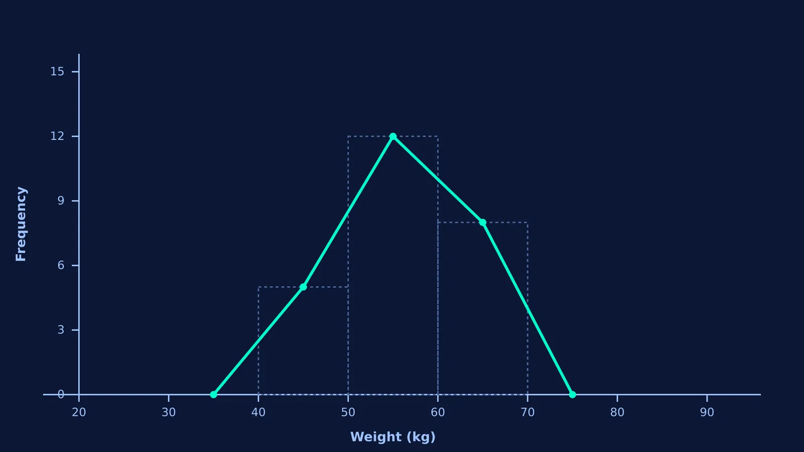
First, determine your given class intervals and frequencies. Imagine you have three actual classes: 40 to 50 kg (frequency 5), 50 to 60 kg (frequency 12), and 60 to 70 kg (frequency 8).
Next, add your imaginary zero-frequency classes at the start and end: 30 to 40 kg (frequency 0) and 70 to 80 kg (frequency 0).
Finally, calculate the Class Mark (midpoint) for every interval and write them as coordinate points (x, y):
Imaginary start: midpoint 35, frequency 0. Point: (35, 0)
First class: midpoint 45, frequency 5. Point: (45, 5)
Second class: midpoint 55, frequency 12. Point: (55, 12)
Third class: midpoint 65, frequency 8. Point: (65, 8)
Imaginary end: midpoint 75, frequency 0. Point: (75, 0)
You simply plot these coordinate pairs and join them with straight lines. You now have a perfect frequency polygon without drawing a single histogram bar.
Understanding how to group and graph data is the foundation of modern statistics. To explore how graphing techniques evolved, you might want to look at how to look at data before testing it with box plots, or explore how adding to or scaling data changes the mean and variance.