

On this page
In the summer of 1654, French writer Antoine Gombaud, known as the Chevalier de Méré, approached mathematician Blaise Pascal with a gambling dilemma (Devlin, 2010). De Méré had made steady profits betting he could roll at least one six in 4 throws of a fair die. Seeking larger stakes, he began betting on rolling at least one double-six in 24 throws of two dice. By his calculations, both bets offered equal odds. Yet according to gambling lore and Pascal's letters, de Méré found himself losing money on the two-dice game (Hald, 1990).
While later historians like Oystein Ore noted that detecting a 0.86% deficit through casual salon play would require thousands of trials, de Méré suspected a theoretical flaw and concluded that arithmetic was self-contradictory. Pascal forwarded the puzzle to Pierre de Fermat on 29 July 1654, beginning the correspondence that founded modern probability theory (Hald, 1990; Gorroochurn, 2011). Their exchange showed that de Méré had fallen for a classic illusion: assuming probabilities across successive trials scale linearly.
Why did Chevalier de Méré think the two bets were equal?
De Méré relied on a proportional rule of thumb common among 17th-century gamblers (Hald, 1990). A fair die has 6 outcomes, giving a 1/6 chance of rolling a six. De Méré assumed rolling 4 times yielded an accumulated chance of 4 × (1/6) = 4/6, or 2/3. Because 2/3 exceeds 1/2, betting at even money produced regular profits.
With two dice, the sample space expands to 36 outcomes, with a double-six occurring with probability 1/36. De Méré observed that 24 throws out of 36 matched his original ratio: 24/36 = 4/6 = 2/3 (Hald, 1990). He assumed 24 throws of two dice offered the exact same winning margin.
This intuition fails because separate throws are not mutually exclusive. Probabilities add directly only when events cannot happen together. Because a player can roll a six on multiple throws in the same sequence, adding probabilities overcounts overlapping successes. If addition held, rolling 6 times would yield 6 × (1/6) = 1, falsely guaranteeing a six. Understanding this distinction is key to separating independent and mutually exclusive events.
How does the complement method calculate the exact probabilities?
Instead of adding overlapping winning combinations, Pascal and Fermat evaluated the opposite outcome: rolling zero sixes, known as the complement method (Wolfram MathWorld).
Because all probabilities in a sample space sum to 1, the probability of at least one success equals 1 minus the probability of zero successes.
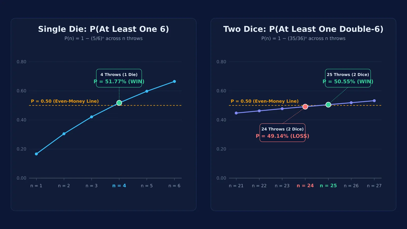
For a single die in 4 throws, the chance of failing to roll a six on any single throw is 5/6. Over 4 independent throws, the probability of failing every time is: P(no six in 4 throws) = (5/6)⁴ = 625 / 1296 ≈ 0.4823.
Subtracting this failure rate from 1 gives the exact win probability: P(at least one six in 4 throws) = 1 − (5/6)⁴ = 671 / 1296 ≈ 0.5177.
This 51.8% win rate gave de Méré an edge of nearly 1.8% over even money (Wolfram MathWorld).
For two dice in 24 throws, failing to roll a double-six has probability 35/36 per roll. Across 24 independent throws, the probability of never rolling a double-six is: P(no double-six in 24 throws) = (35/36)²⁴ ≈ 0.5086.
Subtracting from 1 gives: P(at least one double-six in 24 throws) = 1 − (35/36)²⁴ ≈ 0.4914.
At roughly 49.1%, the wager is unfavorable, losing nearly 1.7% of the stake per game over time (Wolfram MathWorld).
Why do probabilities fail to scale linearly across multiple trials?
The divergence between 0.518 and 0.491 shows that the cumulative probability function P = 1 − (1 − 1/N)ⁿ is non-linear. Even when the ratio n/N remains fixed at 2/3, the winning probability drops as the number of possible outcomes N increases (Gorroochurn, 2011).
As N approaches infinity with n = (2/3)N: lim (1 − 1/N)^{(2/3)N} = e^(−2/3) ≈ 0.5134.
This gives a limiting success rate of 1 − e^(−2/3) ≈ 0.4866, or 48.7%. As N increases from 6 to 36 and beyond, holding n/N = 2/3 causes success to decline toward 48.7%.
To find the minimum throws needed for a favorable bet (P > 0.50), we solve (1 − 1/N)ⁿ < 0.50: n > ln(2) / [−ln(1 − 1/N)].
For 1 die (N = 6): n > ln(2) / [−ln(5/6)] ≈ 3.80, so 4 throws suffice.
For 2 dice (N = 36): n > ln(2) / [−ln(35/36)] ≈ 24.60, so 24 throws falls short and 25 are required.
This non-linear curve is essential when converting odds in favour into probabilities.
How can you solve "at least one" probability questions in competitive exams?
Exam problems in JEE Main and Advanced frequently test this additive fallacy (Gorroochurn, 2011). When approaching questions involving repeated trials, apply this four-step framework:
Identify the trigger: Spot phrases such as "at least one success" or "at least once".
Define the complement: Formulate the scenario where zero successes occur.
Compute the complement: For n independent trials with failure probability q = 1 − p, evaluate P(zero) = qⁿ.
Subtract from unity: Calculate P(at least one) = 1 − qⁿ.
Worked example: Find the minimum throws of a fair die needed so that the probability of rolling at least one six exceeds 90%.
Target: P(at least one 6) > 0.90.
Complement form: 1 − (5/6)ⁿ > 0.90, giving (5/6)ⁿ < 0.10.
Logarithms: n ln(5/6) < ln(0.10), so n [ln(6) − ln(5)] > ln(10).
Numerical check: Using ln(1.2) ≈ 0.1823 and ln(10) ≈ 2.3026, n > 2.3026 / 0.1823 ≈ 12.63.
Answer: At least 13 throws are required.
This framework avoids the traps analyzed in common probability reasoning mistakes in JEE maths. The Fermi Problem Library features worked problems with a step-by-step solver that explains the reasoning rather than printing an answer, helping students master multi-stage probability. To build conceptual foundations across topics, the Fermi Concept Library covers every concept in mathematics with its own lesson and its place in the map.


