On this page
Electric current is rarely a steady flow; it fluctuates when switches close, lightning strikes, or capacitors discharge. When the current changes over time, finding the total charge delivered to a component requires looking at the entire history of the flow, rather than a single snapshot.
According to OpenStax *University Physics Volume 2*, electric current is the time derivative of charge, expressed as I = dQ/dt. Rearranging this gives dQ = I dt. To find the total charge transferred over a period, you integrate the current with respect to time: Q = ∫ I(t) dt.
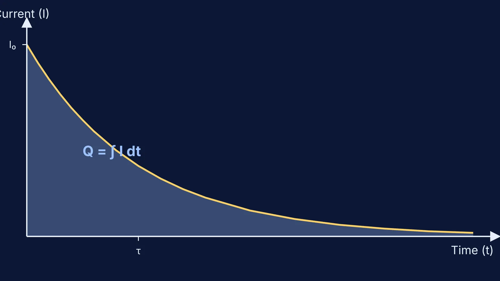
In calculus, a definite integral represents the geometric area under a curve. Therefore, the area between the current plot and the time axis equals the net charge (Q) in coulombs. If you have concept gaps in how integrals translate to physical areas, the Fermi Concept Library maps out these connections, bridging the gap between equations and graphs.
What does the area under a current-time graph represent?
The area under an I-t graph represents the total electric charge that has flowed through a cross-section of a circuit during that specific time interval.
The unit of current is the ampere (A), defined as one coulomb per second (C/s). The unit of time is the second (s). When you multiply the vertical axis (amperes) by the horizontal axis (seconds) to find area, the seconds cancel out: (C/s) × s = C. This confirms that the area measures coulombs.
If the current is a constant direct current (DC), the graph is a horizontal line. The area is a rectangle: I × t. However, most exam problems involve varying currents. Just as converting PV, PT and VT graphs of ideal gas processes requires reading the area for work done, an I-t graph requires reading the area for charge.
How do you find charge from a triangular pulse?
Many transient events, such as a sensor signal or a short circuit, are modelled as triangular pulses. You do not need calculus if the graph is built from straight lines; basic geometry works perfectly.
Imagine a current that starts at 0 A, rises steadily to a peak of 10 A in 2 seconds, and then drops back to 0 A over the next 3 seconds. This mimics an electrical fault where current spikes. The shape is a single triangle with a 5-second base and a 10 A height.
Using the standard geometric formula for the area of a triangle: Area = 1/2 × base × height Q = 1/2 × 5 s × 10 A = 25 C
The total charge delivered by this pulse is 25 coulombs. If the pulse shape were a trapezoid—such as holding steady at 10 A for an extra 2 seconds before dropping—you would split the area into a central rectangle and two side triangles to find the total charge.
How do you calculate charge for a discharging capacitor?
In RC circuits, current does not change linearly. When a capacitor discharges through a resistor, the charge leaves rapidly at first, then slows down.
According to Section 10.5 of OpenStax *University Physics*, the current in a discharging RC circuit follows an exponential decay curve: I(t) = I₀e^(−t/τ). Here, I₀ is the initial current, and τ is the time constant of the circuit, equal to the resistance multiplied by the capacitance (τ = RC).
To find the total charge initially stored in the capacitor, we integrate this current from t = 0 to t = ∞: Q = ∫ I₀e^(−t/τ) dt (from 0 to ∞)
The antiderivative of e^(−t/τ) is −τe^(−t/τ). Evaluating this from zero to infinity: Q = I₀ [−τe^(−∞) − (−τe⁰)]
Since e^(−∞) approaches 0 and e⁰ = 1: Q = I₀(0 + τ) = I₀τ
Because I₀ = V/R and τ = RC, this simplifies to Q = (V/R) × RC = CV. This perfectly matches the standard formula for total charge stored on a capacitor's plates. The area under the decay curve accounts for every electron that leaves the capacitor. Similar limit rules apply when calculating transient states, such as inductors at t = 0 and t = ∞. If you drop a minus sign while setting up these limits, the step-by-step solver in the Fermi Problem Library explains the reasoning rather than printing an answer.
How do you set up the integral for charge?
Whether you are integrating over n periods for an alternating current or evaluating a single pulse, use this framework to avoid common mistakes:
Verify the limits: Determine when the current starts and stops flowing. These are your integration bounds.
Check the signs: If the current dips below the time axis, the area is negative, meaning the charge flows in the opposite direction.
Choose your method: If the function is a polynomial or exponential, use calculus. If it is made of straight lines, use triangles and rectangles.
Scale the units: Ensure the product of the axes resolves to amperes × seconds to yield standard coulombs.