

On this page
Have you ever looked at a probability problem involving a shooter hitting a target or a student taking a test, and wondered how to find the chance of "at least one" success? If you add up the probabilities of exactly one hit, exactly two hits, exactly three hits, and so on, you will run out of time. There is a faster way.
What is the complement rule?
In statistics, the complement of an event is everything that is *not* that event. According to OpenStax's *Introductory Statistics*, if P(A) is the probability of an event happening, its complement is P(A'), and their sum is always 1.
When an exam question asks for the probability of "at least one" success, its exact complement is very simple: zero successes.
P(at least one) = 1 − P(none)
As OpenStax notes for binomial distributions, finding the probability of "at least one" success in independent trials is much faster when you subtract the probability of zero successes from 1. Instead of calculating several independent events, you only calculate one: the chance of failing completely.
If you are struggling with selection problems with combinations, this trick is your first line of defence. It simplifies complex counting problems into a single, manageable subtraction.
How many trials to cross a target probability?
Examiners often flip the question to test your algebra. They give you the success rate and ask: *How many trials (n) are needed to ensure the probability of at least one success is greater than 0.99?*
Let’s look at a classic JEE Main problem. A shooter has a probability of 0.2 of hitting a target on any single shot (p = 0.2).
First, find the probability of missing a single shot: 1 − 0.2 = 0.8
If the shooter fires 5 shots, the probability of missing all 5 independent shots is: 0.8 × 0.8 × 0.8 × 0.8 × 0.8 = 0.8⁵ = 0.32768
Using the complement rule, the chance of hitting the target at least once in 5 shots is: 1 − 0.32768 = 0.67232
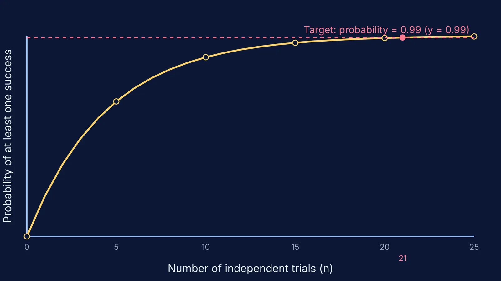
But what if we want the probability of at least one hit to be greater than 0.99? We want: 1 − P(none) > 0.99 1 − (0.8)ⁿ > 0.99 0.01 > (0.8)ⁿ
To solve for n, take the logarithm of both sides: log(0.01) > n × log(0.8)
Since log(0.8) is a negative number, the inequality sign flips when you divide by it: n > log(0.01) / log(0.8)
Using base 10 logarithms, log(0.01) = −2 and log(0.8) ≈ −0.0969: n > −2 / −0.0969 ≈ 20.6
Because n must be a whole number, the shooter needs 21 shots to be certain the probability of hitting the target at least once is greater than 0.99. This logic applies strictly whether you are drawing cards, rolling dice, or dealing with probability problems with and without replacement.
How does the complement rule work with cards?
Beyond binomial targets, the complement rule is essential for problems involving dice, cards, or combinations. Consider a standard deck of 52 cards. If you draw three cards at random, what is the probability of getting at least one heart?
You could calculate the probability of getting exactly one heart, exactly two hearts, and exactly three hearts, adding them all together. However, finding the complement is much simpler: what is the probability of getting zero hearts?
There are 13 hearts in a deck, meaning there are 39 cards that are not hearts. The probability of drawing three cards that are not hearts is calculated by taking the combinations of those 39 cards over the total combinations of 52 cards.
Using combinations, the probability of zero hearts is (39 choose 3) divided by (52 choose 3). This is (39 × 38 × 37) / (52 × 51 × 50), which simplifies to 703 / 1700.
Therefore, the probability of drawing at least one heart is simply 1 minus (703 / 1700), which equals 997 / 1700. This single subtraction saves you from calculating three separate combination scenarios and adding complex fractions.
This is exactly why exam setters love "at least one" questions. They are designed to punish students who try to calculate every positive outcome manually. By recognising the phrase "at least one", you can immediately pivot to calculating the chance of "none" and subtracting it from 1. The time you save on these calculations can be crucial during competitive exams where every minute counts.
How does this apply to exam preparation?
This mathematical rule holds a hidden lesson for exam preparation. If you have a probability of 0.2 of solving a hard maths problem correctly on your first attempt without looking at the solution, your probability of failing is 0.8.
If you stop there, the odds are against you. But if you try 5 different problems of the same type, your probability of solving *at least one* independently jumps to 0.67. The curve in our graph shows this visually: as the number of attempts (n) grows, the probability of complete failure drops exponentially towards zero. Keep practising until n is high enough to make success almost certain.
If you find yourself making reasoning mistakes in probability, try stepping through the logic in the Fermi Problem Library. The step-by-step solver breaks down the 1 − P(none) rule, so you can see exactly where the numbers come from rather than just memorising the final formula.


