

On this page
Most physics students encounter circuits only as textbook schematics. Arrowed loops represent current, parallel lines denote capacitors, and jagged lines stand in for resistors. When faced with physical hardware or practical exams, many struggle to connect those symbols to real components. Building low-voltage circuits at home bridges this divide between abstract formulas and physical reality.
What makes low-voltage bench circuits safe for home experiments?
Electrical safety depends on the voltage driving current across the resistance of the human body. Under standard 29 CFR 1910.303(g)(2)(i) published by the Occupational Safety and Health Administration, live electrical parts operating below 50 V direct current (DC) or alternating current (AC) do not require guarding against accidental contact. Dry human skin presents an electrical resistance between 1,000 Ω and 100,000 Ω, so a 9 V battery drives no more than a harmless fraction of a milliampere through fingers.
Working with 5 V from a USB charger or a 9 V alkaline battery stays safely below this threshold. Mains electricity from wall sockets (230 V in India) must never be connected to student breadboards. Bare lithium-ion cells should also be avoided because accidental short circuits draw high discharge currents. Low-voltage bench experiments let students explore physics without anxiety, following habits that help children learn without adding pressure.
Why do textbook circuit diagrams fail to build physical intuition?
Paper diagrams often conceal how circuits function. In the *American Journal of Physics*, Paula Vetter Engelhardt and Robert J. Beichner developed the 29-item DIRECT diagnostic assessment (Engelhardt and Beichner, 2004) across 1,135 high school and university physics students. They found students hold persistent misconceptions, such as treating a battery as a constant current source rather than a supplier of constant potential difference, or believing current is consumed along a loop.
Physical measurement dismantles these flawed models. Placing a multimeter ammeter in series before and after a resistor proves charge is conserved, while checking parallel branches confirms both receive equal supply potential. This hands-on habit also builds the diagnostic skills needed when measuring resistivity with a V–I graph during laboratory practicals.
How can you verify Ohm's law with a breadboard and multimeter?
Ohm's law states that current through an ohmic conductor is directly proportional to the potential difference across it at constant temperature: V = IR.
Place a 1 kΩ resistor across the central divider of a solderless breadboard.
Connect a variable DC supply (or a 9 V battery regulated with a 10 kΩ potentiometer).
Set a multimeter to DC volts across the resistor to measure potential difference V.
Place an ammeter in series with the positive lead to record current I.
Record voltage and current across five potentiometer settings from 1.5 V to 8.0 V.
Plotting voltage V against current I yields a straight line through the origin whose slope gives resistance R. Comparing this slope to the nominal rating reveals real-world contact resistance and component tolerances.
How do you measure capacitor charging and the RC time constant?
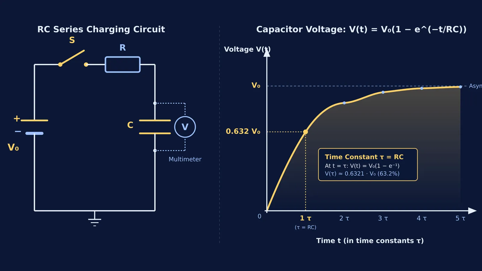
In an RC series circuit, a capacitor charges exponentially: V(t) = V₀(1 − e^(−t/RC)), where V₀ is supply voltage, R is resistance, and C is capacitance. The time constant τ = RC marks the interval required to reach roughly 0.632 of supply voltage, determined by 1 − 1/e.
You can track this transition with a multimeter and a stopwatch:
Pair a 10 kΩ resistor with a 1,000 µF capacitor to yield a 10.0-second time constant: τ = (10,000 Ω) × (0.0010 F).
Discharge the capacitor through a jumper resistor before starting.
Close the circuit switch and log capacitor voltage every 5 seconds up to 30 seconds.
At t = 10.0 s, the multimeter reads approximately 5.69 V on a 9.0 V source (0.632 of V₀). You can analyze how resistance shapes charging curves in our guide to transient charging curves in RC circuits.
How do sensor circuits demonstrate potential dividers?
A potential divider splits supply voltage across two series resistances: V_out = V_in × (R₂ / (R₁ + R₂)). Replacing one resistor with a sensor demonstrates how hardware responds to the physical world.
A Light Dependent Resistor (LDR) drops in resistance as incident light frees charge carriers. In dim light, an LDR measures 50 kΩ to 100 kΩ; in bright light, it falls below 1 kΩ. Paired with a 10 kΩ fixed resistor across 5 V, the output voltage swings between 4.5 V in darkness and under 0.5 V in bright light, illustrating how light sensors automate circuits.
How should students combine physical kits with digital simulations?
Physical circuits teach tactile assembly and component quirks, but real parts include unmodelled friction like lead resistance and supply voltage sag. A study by Noah D. Finkelstein and colleagues (Finkelstein et al., 2005) showed that students using circuit simulations developed stronger conceptual models than those using physical kits alone, mastering hands-on wiring faster afterwards.
Research by Zacharias C. Zacharia (Zacharia, 2007) across 88 undergraduate physics students confirmed that combining simulations with physical lab work produced higher comprehension than physical equipment alone. Virtual tools reveal invisible electron drift, while breadboards test real tolerances.
When component quirks obscure the core physics, the Fermi Simulation Lab provides interactive simulations for ideas that are easier to see than to read, letting you observe ideal circuits before wiring breadboards.
If bench readings diverge from theory, Fermi's AI tutor can work out what you already know and build a plan for the session, guiding you through diagnostic measurements to pinpoint where the discrepancy arose.


