

On this page
In high school physics, electric circuits often feel like simple puzzles solved by reducing series-parallel resistors or tracing an informal loop. In a first-year undergraduate engineering course—typically structured around the All India Council for Technical Education (AICTE) Basic Electrical Engineering curriculum—circuits scale up to multi-node networks, dependent sources, transient responses, and complex AC steady-state analysis. Transitioning successfully requires replacing intuitive guesswork with systematic network analysis and regular, structured problem practice.
Why is first-year basic electrical engineering harder than school physics?
The difficulty of first-year electrical engineering rarely stems from higher mathematics; it stems from persistent conceptual gaps carried over from school science. In a study in the *American Journal of Physics*, researchers Paula Vetter Engelhardt and Robert J. Beichner evaluated students using the 29-item DIRECT inventory. Even after completing formal physics courses, students held persistent misconceptions—believing a battery supplies a fixed current regardless of the load, confusing electric potential with current, and reasoning sequentially as if downstream changes never affect upstream branches.
More recently, a 2025 study led by María José Canet and colleagues in *IEEE Transactions on Education* identified Ohm's law and potential difference as true "threshold concepts" for first-year engineering students. The authors found that until students stop treating voltage as an isolated component's property and understand it as a spatial potential difference between two coordinates, advanced theorems remain bewildering. Revisiting the basics of combination of resistors helps clarify how series and parallel branches constrain charge before tackling larger networks.
How do you transition from loop guessing to systematic nodal analysis?
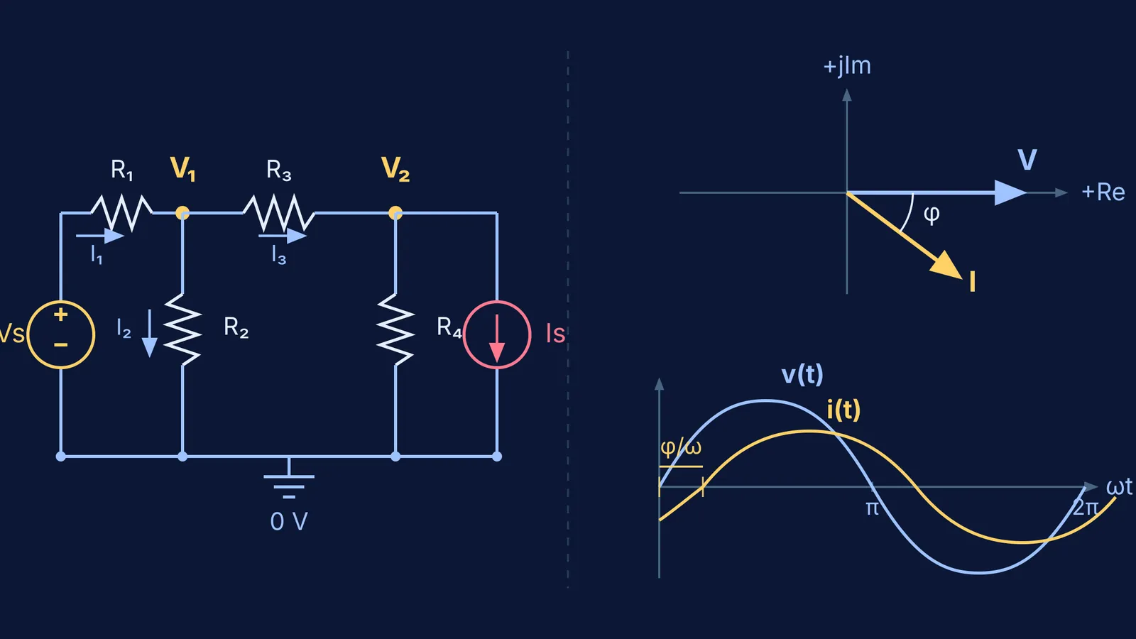
School physics often encourages students to sketch arbitrary Kirchhoff's Voltage Law (KVL) loops across circuit windows. In a network with four interconnected branches, this habit creates messy simultaneous equations and sign errors. Professional engineers use systematic Nodal Analysis because it scales cleanly and generates standard matrix equations.
In nodal analysis, you select one junction as the reference ground node (0 V) and write Kirchhoff's Current Law (KCL) equations setting the sum of branch currents leaving each non-reference node to zero:
Designate a continuous bottom wire as the reference node (0 V).
Label unknown junction voltages as V₁, V₂, and so on.
Express each branch current as (V_node − V_neighbour) / R.
Solve the linear algebraic system for node potentials.
Consider a practical example: a junction V₁ connects to a 20 V DC source through a 5 Ω resistor, to ground through a 10 Ω resistor, and to an adjacent node fixed at 8 V through a 2 Ω resistor. Expressing outward branch currents:
(V₁ − 20) / 5 + V₁ / 10 + (V₁ − 8) / 2 = 0
Multiplying by 10 gives 2(V₁ − 20) + V₁ + 5(V₁ − 8) = 0. Expanding yields 8V₁ − 80 = 0, resolving to V₁ = 10 V in three lines. Mastering the node potential method eliminates loop-variable guesswork.
When networks include dependent sources and choosing between mesh or nodal analysis is unclear, the Fermi Problem Library provides worked problems with a step-by-step solver that explains the reasoning rather than printing an answer.
How should you practice AC circuits and phasor calculations?
Moving from direct current (DC) to alternating current (AC) represents the next major conceptual leap. In university engineering, you must calculate active power, reactive power, and power factor across complex networks.
Rather than solving time-domain differential equations for every inductor and capacitor, circuit theory transforms sinusoidal waveforms into the frequency domain using complex phasors. Every sinusoidal voltage v(t) = V_m cos(ωt + θ) becomes a phasor V = V_rms ∠θ, while components become complex impedances:
Resistors: Z_R = R
Inductors: Z_L = jωL (where j = √−1)
Capacitors: Z_C = 1 / (jωC) = −j / (ωC)
With complex impedances, all DC network laws apply unchanged. Reviewing AC circuits and phasors solidifies impedance triangles and phase angles. For electromagnetic topics where phase shifts and alternating waveforms are hard to picture on paper, the Fermi Simulation Lab offers interactive simulations for ideas easier to see than read.
What is an effective daily problem-solving routine for engineering circuits?
Basic electrical engineering is a procedural skill; reading solved textbook problems creates an illusion of competence. In a study published in *Cognition and Instruction*, Paul Chandler and John Sweller showed that novice circuit learners experience severe cognitive load when splitting attention between separate diagrams and text explanations.
To address this, research by Tamara van Gog, Liesbeth Kester, and Fred Paas in *Contemporary Educational Psychology* demonstrated that using "example-problem pairs"—studying a worked solution immediately followed by solving a similar problem—reduces mental effort and accelerates schema acquisition in circuit analysis.
A 45-minute daily routine based on this finding:
15 minutes of worked example study: Deconstruct one textbook problem, noting the reference node and branch equations.
20 minutes of paired practice: Close the book and solve a matched problem with different numerical values without looking at steps.
10 minutes of self-auditing: Verify power conservation; total power generated by active sources must equal power dissipated by resistors (∑ P = 0).
When reviewing earlier concepts connecting school physics to university engineering, the Fermi Concept Library maps every concept in physics, chemistry, biology, mathematics and computing, each with its own lesson and its place in the map.


