

On this page
In introductory calculus classes across CBSE Class 12 and JEE preparation, students learn to find the slope of a curve by differentiating its equation. They memorize the point-slope formula for a tangent line, invert the slope for the normal line, and work through textbook exercises. Yet when asked to sketch these lines on an unfamiliar graph, many hesitate. What seems straightforward on paper often disconnects from geometry: why does a tangent touch without cutting, how can it pass through an inflection point, and what happens when the slope drops to zero? Moving a point along a live mathematical curve transforms static rules into dynamic intuition.
Why do students struggle with tangents and normals?
Most learners first meet tangents in Euclidean circle geometry, where a tangent touches a curve at exactly one point and never crosses it. When students transition to differential calculus, this early intuition becomes a stumbling block. In seminal research in Educational Studies in Mathematics, David Tall and Shlomo Vinner (1981) showed how intuitive "concept images" conflict with formal "concept definitions." In The Journal of Mathematical Behavior, Irene Biza and Theodossios Zachariades (2010) tracked undergraduate calculus students. Many rejected valid tangents whenever a line crossed the curve at an inflection point or intersected elsewhere, clinging to circle-geometry rules.
Solving calculating tangents and normals with derivatives purely by algebra leaves these barriers hidden. You can find dy/dx and write y − y₀ = m(x − x₀) without picturing how the lines behave as the contact point moves.
How does predicting where dy/dx = 0 change your understanding?
Passive watching rarely corrects an ingrained misconception. Active learning research shows that committing to a prediction before seeing the result creates cognitive contrast that locks in understanding.
In a meta-analysis of 50 studies in the International Journal of Interactive Mobile Technologies, Dadang Juandi and colleagues (2021) examined dynamic mathematics software across secondary and higher education. They found an overall effect size of 1.07, meaning an average student using interactive tools outperformed 84% of conventionally taught peers. Gains peaked when students worked individually, testing mathematical conjectures on screen.
Predicting where dy/dx = 0 before moving a slider turns observation into hypothesis testing. You identify where the slope should flatten, then drag the point to verify your prediction against the live graph.
The Fermi Simulation Lab provides interactive simulations for the ideas that are easier to see than to read, letting you drag points across curves, test slopes, and observe rates of change in real time.
What happens to the normal line when the tangent is horizontal?
The normal line at (x₀, y₀) is perpendicular to the tangent line. When the tangent slope m = f'(x₀) is non-zero, perpendicular slopes satisfy m₁ × m₂ = −1. The normal slope is therefore m_n = −1/m, giving:
y − y₀ = −(1 / f'(x₀)) (x − x₀)
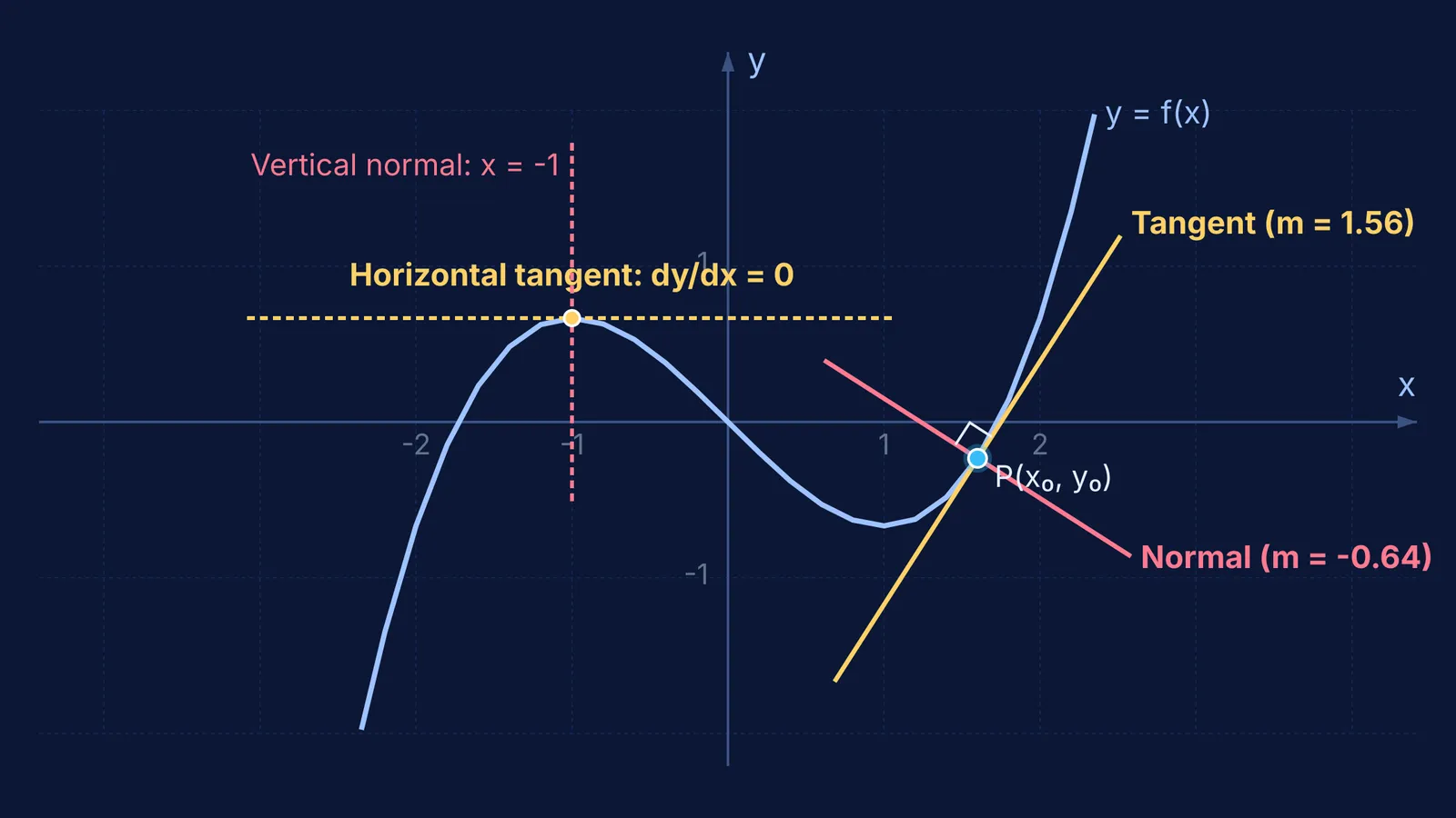
This rule creates an edge case at stationary points. When dy/dx = 0, the tangent line is horizontal (y = y₀). Dividing by zero leaves the normal slope undefined in algebra, but the geometry is clear: as the tangent levels flat, the normal swings vertical to become x = x₀.
Understanding this shift is essential for analyzing maxima, minima and turning points and testing differentiability at sharp corners.
How can you test curves with an interactive workflow?
To make tangent and normal analysis a reliable habit, follow this four-step interactive routine whenever you explore a new function:
Solve turning points: Differentiate y = f(x) and set dy/dx = 0 to find where tangents are horizontal.
Predict the geometry: Sketch whether each stationary point is a crest, trough, or inflection.
Drag and test slopes: Move the point along the curve to see the tangent flatten at turning points and steepen elsewhere.
Track the normal: Check that the normal stays at 90° to the tangent, turning vertical whenever the tangent lies flat.
Consider the cubic curve y = (1/3)x³ − x. Differentiating yields dy/dx = x² − 1. Setting x² − 1 = 0 gives horizontal tangents at x = −1 and x = 1. At x = −1 (where y = 2/3), the tangent is y = 2/3 and the normal is x = −1. At x = 1 (where y = −2/3), the tangent is y = −2/3 and the normal is x = 1. At the inflection point (0, 0), dy/dx = −1: the tangent cuts through the curve with slope −1, while the normal crosses at slope +1.
If you get stuck on derivations or sign errors in coordinate geometry sets, the Fermi Problem Library offers worked problems with a step-by-step solver that explains the reasoning rather than printing an answer.


